Truss Element |
 
|
Truss Element |
|
The truss element has 3 translational degrees of freedom at each node, and deforms only in the axial direction (it does not deform in bending or torsion). As it does not solve for nodal rotations, the connection at each node is essentially a pure hinge. The axial force penalty term is retained making the truss element a 7-DOF hybrid finite element with two end nodes. The truss element is designed specifically for modelling structures which have very low levels of structural bending stiffness (such as mooring chains) and is essentially a simplified version of the standard beam-column element employed by Flexcom.

7-DOF Truss Element
Modelling of flexible lines can be quite challenging, especially in severe dynamic environments, where there is a tendency for the lines to go slack intermittently. Due to the low structural bending stiffness, the standard beam column elements employed by Flexcom are not well suited to this type of scenario. When the beam element attempts to solve for nodal rotations, the lack of bending resistance can lead to a solution indeterminacy. In such circumstances, truss elements offer both increased solution robustness and increased computational efficiency. Faster computation times are due to the reduced number of degrees of freedom in the model, and the ability to run at larger time-steps (particularly when lines go slack).
The general finite element formulation for truss elements is similar to that of beam elements, which has been discussed in some detail in the preceding articles. For example, each truss element has its own Convected Axis System and the Equations of Motion are applied in a consistent manner regardless of whether a model consists of beam elements, truss elements or a combination of both. Due to the fewer active degrees of freedom, there are some differences in the formation of the constitutive matrices for truss and beam elements. The following sections present the truss element formulation in more detail.
Note that Truss Elements supersede the Mooring Line modelling feature which is now outdated. In this older approach, the mooring line is modelled using a combination of standard beam elements interspersed with hinge elements. While this hybrid approach offers increased solution robustness over traditional beam models, it represents an inefficient solution procedure with the model containing many more elements than an equivalent truss element model.
The local deformation vector at any point along the element, udef(x), is related to the nodal deformation vector of the element, dnd, by the matrix of shape functions, [N(x)].
![]() (1)
(1)
The truss element undergoes axial deformation only so the element shape is a straight line between the two end nodes. Therefore linear shape functions are used to interpolate for deflections at points intermediate to the end-nodes.
 (2)
(2)
where:
![]() (3)
(3)
![]() (4)
(4)
are the linear interpolation (shape) functions for the truss element and L is the element length. Note that these differ from the shape functions that are used for a beam-column element, in particular the truss element uses linear functions to interpolate for the lateral deflections, v(x) and w(x), whereas the beam-column element uses cubic polynomial (Hermitian) interpolation functions.
The linear stiffness matrix [KL] is defined as:
![]() (5)
(5)
Here [D] is the constitutive matrix which relates the stress and strain vectors. For a truss element with only axial deformation, the constitutive matrix contains only a single element, which is the axial stiffness EA. Note that in the current version of Flexcom, EA must have a constant (linear) value. Non-linear axial stiffness will be supported in a future version.
[B(x)] is the matrix of functions relating the linear strain to the nodal deformation vector.
The linear stiffness matrix [KL], including the axial penalty terms, may be derived as:
 (6)
(6)
For beam-column elements, γ1 is related to the ratio of the bending to axial stiffness (γ1 = EI / EA.L2). However as truss elements have no bending stiffness a fixed value of γ1 = 1 x 10⁻⁵ is used (the same value is used for spring elements which have essentially the same form of linear stiffness matrix). The parameter ρ1 is a flexibility coefficient with a default value of 0.001.
The geometric stiffness matrix [KG] is defined as:
![]() (7)
(7)
Here [Aσ] is a 2x2 matrix based on effective tension T:
![]() (8)
(8)
and [G(x)] is the matrix that relates a vector of slopes to the nodal deformation vector. [G(x)] is found by differentiating the second and third rows of the shape function matrix [N(x)] with respect to x and is given by:
 (9)
(9)
The geometric stiffness matrix [KG] may be derived as:
 (10)
(10)
Note that the above exact form of the geometric stiffness matrix assumes that the effective tension T is constant along the element. This is not the case in general, so the geometric stiffness matrix is found using numerical integration.
It is also important to note that the contribution from the geometric stiffness matrix is included only if T is positive, as flexible lines (modelled using truss elements) cannot carry compressive loads. If T is negative at any specific integration point, the geometric stiffness contribution is assumed to be zero. Intuitively one would expect that a truss element should never experience effective compression, but it is mathematically possible in a numerical model. Refer to Compression in Truss Elements for further discussion on this topic.
The first solution iteration of an initial static analysis is a special case. Geometric stiffness relies on the presence of a positive effective tension, but no effective tension results are formally computed until after the first solution iteration has been completed.
•If you are modelling a catenary section, using either the *CABLE or *LINES keywords, the Cable Pre-Static Step is invoked. Using cable catenary equations, this step provides the finite element solver with approximate nodal coordinates, and it also provides an estimation of the effective tension in the line. This tension value ensures that the geometric stiffness contribution is included in the first solution iteration.
•If you are modelling a straight section, using either *NODE/*ELEMENT or *LINES keywords, Flexcom automatically assumes a nominal effective tension value of 1N (or 1lbf) to facilitate the inclusion of a token geometric stiffness contribution. This is generally sufficient to prevent a solution indeterminacy in the initial static analysis. If not however, then you could (i) add some node springs of very low stiffness, or (ii) attempt to solve the model quasi-statically rather than statically, perhaps including a small level of damping to aid numerical stability. In some circumstances, it may even be possible to model the straight section as a catenary by slightly increasing the line length or offsetting one of the end points - even a very minor adjustment will activate the Cable Pre-Static Step and if a catenary profile is successfully computed, this will ensure a realistic effective tension distribution is available for the first solution iteration.
The initial displacement matrix, [KD], as presented in Equations of Motion (Eq.3) for beam elements, is not constructed for a truss element. This aspect of the finite element formulation is only meaningful when bending and torsional degrees of freedom are active and so is reserved for beam elements only. It is not possible to explicitly specify a stress-free orientation for a truss element and so both (i) the specification of V and W vectors under the *LINES or *ELEMENT keywords and (ii) the discussion around Undeformed Versus Initial Positions are not relevant for truss elements.
The mass matrix [M] is defined as:
![]() (11)
(11)
where the density matrix [m] is defined as:
 (12)
(12)
and m is the mass per unit length of the element (which includes contributions from internal fluid and hydrodynamic added mass, if appropriate).
Hence the mass matrix [M] may be derived as:
 (13)
(13)
Note that the above exact form of the mass matrix assumes that the mass (including contributions from internal fluid and hydrodynamic added mass) is constant along the element. This is not the case in general (for example, in the case of changing internal fluid properties or surface-piercing elements), so the mass matrix is found using numerical integration.
The Damping matrix [C] for a truss element is formed as a linear combination of the stiffness and mass matrices in the same way as for beam-column elements. Specifically:
![]() (14)
(14)
The effects of Deformation Mode Damping for a truss element are limited to the axial degree of freedom for the structural stiffness contribution and the bending degrees of freedom for the geometric stiffness contribution. Hence:
![]() (15)
(15)
The table below compares the range of solution parameters available for beam and truss elements.
A limited range of output variables is available for a truss element. In theoretical terms, the generalised stress field presented in Internal Virtual Work Statement (Eq.1) is simplified as:
![]() (16)
(16)
where n is axial force (moments about the local axes are all zero). So the truss element is incapable of presenting any data relating to shear force, bending moment, bending stress or torque. Likewise strain terms such as bending strain, curvature and bend radius are unavailable. For ease of post-processing and compatibility of databases, you may request any of these parameters and the program will simply return zero values rather than issuing an error message.
Note however that although the truss element does not solve for rotational degrees of freedom, results for nodal rotations in DOFs 4, 5 & 6 are available for convenience. These are derived from the element orientations in time and space, which in turn are governed by the translational degrees of freedom of the element end nodes.
Category |
Parameter |
Beam Element |
Truss Element |
|---|---|---|---|
Motion |
DOF1-3 |
ü |
ü |
DOF4-6 |
ü |
ü |
|
Force |
Axial force |
ü |
ü |
Effective tension |
ü |
ü |
|
Shear force |
ü |
û |
|
Moment |
Torque |
ü |
û |
Bending moment |
ü |
û |
|
Stress |
Axial stress |
ü |
ü |
Bending stress |
ü |
û |
|
Von Mises stress |
ü |
ü |
|
Hoop stress |
ü |
ü |
|
Strain |
Axial strain |
ü |
ü |
Curvature |
ü |
û |
|
Bending strain |
ü |
û |
|
Bending radius |
ü |
û |
|
General |
Temperature |
ü |
ü |
Pressure |
ü |
ü |
Results from the truss formulation are validated (Connolly et al., 2025) via code-to-code benchmarking against OrcaFlex, a tool which is well established and highly regarded for mooring system design in the offshore energy industry. Solution accuracy and computational performance are gauged by two separate mooring applications. The main case study considers a heavy steel chain in a catenary mooring configuration, suitable for mooring a traditional semi-submersible platform hosting a large wind turbine. A secondary case considers a weather buoy moored with lightweight polyester rope, highlighting the versatility of the truss element for use in a variety of mooring applications. The truss element is shown to be numerically accurate and dynamically robust.
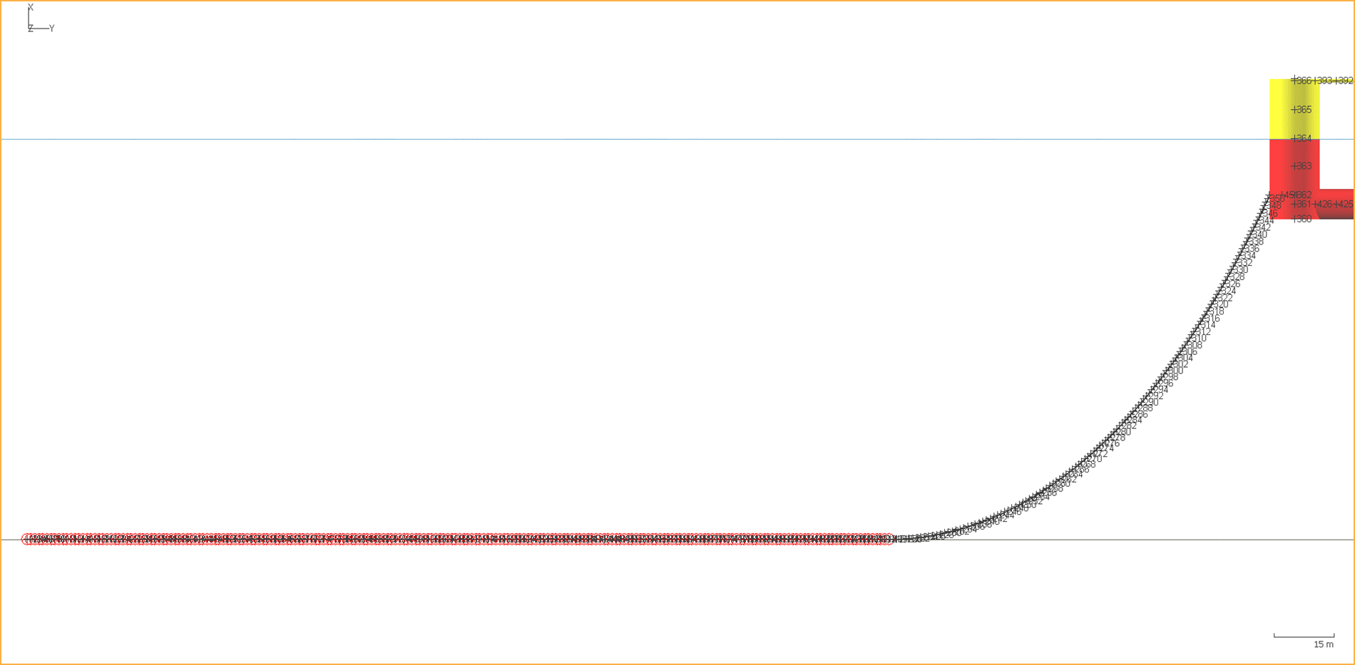
Test Case A IEA 15MW RWT, Heavy Steel Chain Mooring, 100m Water Depth |
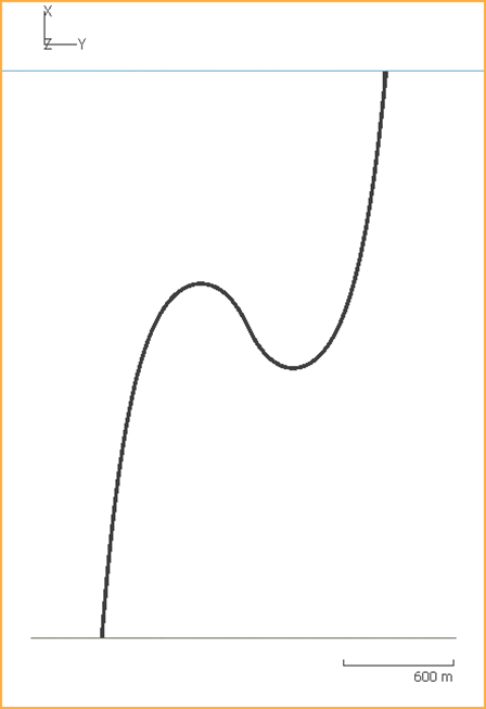
Test Case B M6 Buoy, Light Polyester Rope Mooring, 3100m Water Depth |
|
|
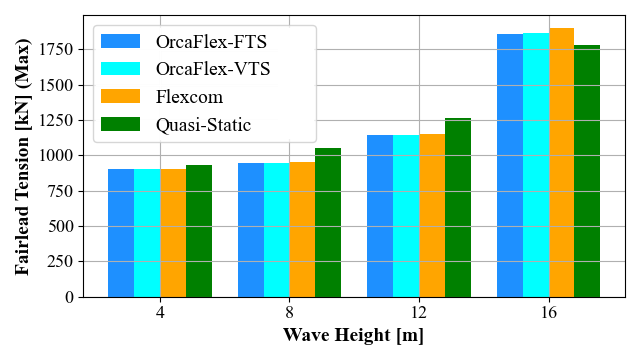
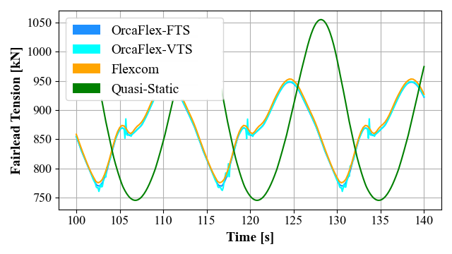
Case A considers the IEA 15MW RWT hosted by the UMaine semi-submersible. Several previous studies (e.g. Allen et al., 2020) examined a fully coupled model of the entire floating system, but this study focuses exclusively on the mooring line and its structural responses. Hence the platform is not explicitly modelled, with representative displacements of the semi-sub applied via RAOs in a decoupled manner instead, and the windward mooring line is examined in isolation. This approach is logical given that (i) in extreme conditions, the turbine is parked, so wind loads are minimised, and wave loads dominate, and (ii) for the purposes of benchmarking the mooring solutions, a displacement driven model ensures that the fairlead motions are identical in both modelling tools. Very close agreement is shown between the dynamic mooring models of Flexcom and OrcaFlex, while some deviations are evident with the OrcaFlex quasi-static catenary solution as expected (given that it ignores inertial and drag effects).
IEA 15MW RWT, Max Fairlead Tension v Wave Height |
IEA 15MW RWT, Fairlead Tension v Time (Hs = 8m) |
|
|
Case B considers the M6 weather buoy, which is located about 350 km west of Ireland. Lying beyond the continental shelf, it is situated in deep water, about 3100 m. It is moored with lightweight polyester rope in a steep-S configuration, to minimise any impact on the wave riding characteristics of the buoy. As per the FOWT model, good agreement is shown between the dynamic mooring models of Flexcom and OrcaFlex. The quasi-static method is not suitable for this model and fails to predict the variations in fairlead tension over time, as hydrodynamic drag plays a significant role in determining the structural response of the lightweight rope due to its very low inertia.
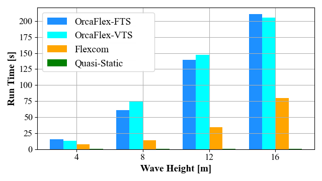
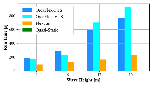
For mooring line modelling, Flexcom 2025.1 appears to be 2-3 times faster than OrcaFlex 11.4. Sample run times for the FOWT (heavy chain) and buoy (light rope) test cases are shown below, comparing OrcaFlex (both fixed and variable time steps), Flexcom and the OrcaFlex quasi-static catenary model. Across all wave heights, Flexcom's truss element model is consistently quicker than the OrcaFlex beam model and run-times are considerably shorter. There are two potential reasons for this. Firstly, the Flexcom truss element is numerically robust and can run at sizeable timesteps regardless of the severity of dynamic excitation. While the OrcaFlex beam model is also robust, the solver either requires smaller timesteps, or takes more iterations to reach convergence, leading to a slower run time overall. Secondly, the truss element has fewer active DOFs, resulting in smaller matrices and reduced solution bandwidth. By default, the beam element includes rotational DOFs in addition to translational, resulting in more equations to solve. The rotational DOFs have been disabled in the benchmarking study to minimise simulation time, but bending effects are still captured to some degree. The quasi-static catenary method is exceptionally quick and run-times for regular wave analysis are practically instantaneous. However, it has some inherent limitations in the formulation which would likely preclude its use in detailed engineering design phases.
IEA 15MW RWT, Run Time v Wave Height |
M6 Buoy, Run Time v Wave Height |
|
|
Interested readers are referred to the official technical publication (Connolly et al., 2025) for full details of the benchmarking study. Although the research was performed by Wood Group, the process was fully open and transparent. Orcina were afforded the opportunity to review the numerical models (and a draft version of the paper) and offer suggestions for improvement. The authors are grateful to Orcina for their professional guidance and timely support regarding the use of their software.
Run-time comparisons were facilitated by command prompt batch files, which ensure consistency and a valid comparison. Each dynamic simulation was performed on its own, with no other simulations competing for CPU resources, affording the solvers a good chance of achieving the quickest possible run time.
Regular wave loading only was considered in the benchmarking study, which assisted with computational efficiency to expedite the research process. Detailed engineering design involves a large load case of random sea loading based on a wave scatter diagram, which is far more computationally intensive than regular wave cases. Hence any run-time savings associated with the truss element would be accentuated.
Please note that this run-time performance exercise was performed in 2024 so the times above may not necessarily reflect the exact computation speeds of the modelling tools as of today. Run-times for other mooring systems may differ also, so this particular benchmark does not represent a definitive statement on the execution speeds of OrcaFlex and Flexcom.
The following were the specifications of the test machine.
Parameter |
Value |
|---|---|
Processor |
Intel(R) Core(TM) i7-10700 CPU @ 2.90GHz |
RAM |
32 GB |
Operating System |
Windows 10 Enterprise, 64-bit |
Flexcom |
Version 2025.1.2 |
OrcaFlex |
Version 11.4d |
•*GEOMETRIC SETS is used to assign structural properties, including those of truss elements.
If you would like to see an example of truss elements used in practice, refer to either E01 - CALM Buoy - Simple or L04 - IEA 15MW RWT.