Flexcom Methodology |
 
|
Flexcom Methodology |
|
Hysteresis generally applies to a pressurised flexible riser after it has been installed and become operational. Flexcom therefore allows the effects of hysteresis to be excluded from an initial series of static or quasi-static analyses (via the *NO HYSTERESIS keyword) so that the initial riser configuration is determined using the depressurised (linear elastic) bending stiffness. The stiffness for the static analysis when this option is selected equals the slope of the last segment in the moment-curvature input data described below. The final computed static configuration is then used as a relative reference from which to switch on the hysteresis stiffness.
The *NO HYSTERESIS keyword allows you to explicitly exclude hysteresis effects from any individual analysis (including dynamic, although this would represent an unusual request). Note that this input is not carried through to any subsequent restart analysis – it must be explicitly specified in every analysis stage in which it is warranted.
Hysteresis can cause the stiffness terms to repeatedly toggle between high pre-slip and low post-slip values during iteration at a particular solution time, which can prevent convergence. The problem is circumvented by solving each time step twice, first with a pre-hysteresis step and then a hysteresis analysis. The pre-hysteresis analysis keeps the stiffness unchanged from the previous time step. The solution of the pre-hysteresis analysis is then used to determine an expected stiffness value based on the rules of hysteresis, that is, pre-slip, post-slip or reversal. The hysteresis analysis resumes the iteration and will decrease the expected stiffness if required, but will not increase an expected post-slip stiffness to a pre-slip value during the iteration. The two successive analyses carry a small computational overhead but ensure convergence of the iteration method at each solution time.
When invoking the hysteresis option in Flexcom, a moment-curvature relationship for the riser under consideration is required. This is specified in the form of a backbone curve which defines the moment experienced by the pipe for increasing values of curvature. The figure below shows an example of a typical backbone curve (and its piecewise linear components).
The elastic curve is based on the depressurised riser and is comparatively small. The friction curve is the main component of the pressurised condition. The large moments on this curve result from the inter-layer friction on the tensile amour layers. The friction curve levels off towards a zero stiffness (slope) for increasing curvatures. The friction curve is determined from test data or a local structural analysis of the riser cross section. The combined curve is the sum of the elastic and friction curves and provides the input data required by Flexcom.

Hysteresis Backbone Curve
The Flexcom hysteresis analysis can handle any arbitrary number of input segments starting from bi-linear (two segments). A close approximation of a smooth backbone curve is usually achieved with approximately five segments as shown above.
An important part of the hysteresis analysis is the decomposition of the backbone curve. This is achieved using an analogous elastoplastic system of parallel springs as shown in the figure below. Each linear segment of the backbone curve is replaced by an elastoplastic stiffness component.

Assembly of Elastoplastic Stiffness Components
The pre-slip stiffness assigned to each spring is based on the difference in the stiffness of adjacent segments as shown in the above figure, e.g. EIh1 = EI1 – EI2. The post-slip stiffness of each spring is zero, i.e. perfectly plastic. The slip curvature of each spring is equal to curvature at the end of the related segment on the backbone curve of the pipe moment. The first segment has the smallest slip curvature and the last (elastic) segment never slips. The pipe bending stiffness at the current time step is the sum of the elastoplastic components. The rules governing each elastoplastic component for two-dimensional bending are described in the next section, followed by their extension to three-dimensions.
The curves on the right-side of the previous figure define the backbone curves of the elastoplastic stiffness components. The moment curvature relationship at each time step is derived from these backbone curves. The hysteresis relationship for an elastoplastic component is defined by:
![]() (1)
(1)
where M denotes the bending moment, EI bending stiffness, κ bending curvature and h is the Nonlinear Material Force intercept with the moment axis as shown below:

Uniaxial Bending Relationship
The values of M, EI, κ and h are iteratively updated at each time step. The moment update is based on the increment of curvature from the previous time step and the expected stiffness as computed from the pre-hysteresis analysis. The moment is clipped if necessary to stay within the elastoplastic limit (±Mslip = ±EIh κslip) and the stiffness is adjusted to take account of the corrected moment. The stiffness generally equals the pre-slip or post-slip values (EIh or 0), or an interim value if the moment changes between elastic and plastic values. The intercept term h is computed from the curvature and moment at the previous time step and the current stiffness. The intercept term maintains continuity of the bending moment as the stiffness changes between pre- and post-slip values. The finite element formulation assembles the intercept term with the global load vector on the right-hand side of the equation of motion as previously described.
The above figure also shows that the slip moment Mslip provides a natural parameter for defining the elastoplastic limit. The bending curvature is not constrained by the elastoplastic relationship but the moment is restricted to stay to between ±Mslip.
An elastoplastic component in a three-dimensional analysis supports biaxial loading with curvature κ = (κy, κz) and moment Mh = (Mhy, Mhz). The figures below show the key concepts of the biaxial elastoplastic methodology.


Biaxial Bending Relationship
The figure on the left shows the riser bending curvature with local components κy and κz. The circle denotes the (initial) slip curvature as the elastoplastic component bends from straight. The figure on the right shows the bending moment of an elastoplastic component with moments Mhy and Mhz. The circle denotes the slip moment of the elastoplastic component. The moment is elastic when inside the circle and plastic when on the boundary. The moment cannot pass outside this circle.
The curve A to G shows an example of the loading. The loading starts from the origin and passes through points A, B and C with an elastic response and continues to point D at the slip boundary. The moment becomes plastic at D and continues along the slip boundary through E until point F. The plastic moment maintains constant magnitude but tracks the direction of the curvature. The curvature reverses at F (magnitude reduces) and the moment returns to inside the slip boundary.
The hysteresis relationship for a biaxial elastoplastic component is defined by:
![]() (2)
(2)
where M, κ and h denote the moment, curvature and intercept vectors and EI is a scalar (symmetric) bending stiffness that applies to both axes.
The values of M, EI, κ and h are iteratively updated at each time step in a similar manner to the uniaxial elastoplastic component. The moment is first updated using the increment of curvature from the previous time step and the expected stiffness from the pre-hysteresis analysis. The magnitude of the updated moment vector is reduced if necessary to stay within the elastoplastic circular limit.
A curvature reversal occurs when:
1.The magnitude of the curvature, |κ|, from the previous time step exceeds the spring slip curvature.
2.The angle, β, between the curvature at the previous time step, κt-1, and current change in curvature, Δκt = κt – κt-1 is between 90º and 270º.
These two conditions are illustrated in the figure below where a series of curvatures are shown at time t = 0, t = 1 and t = 2:
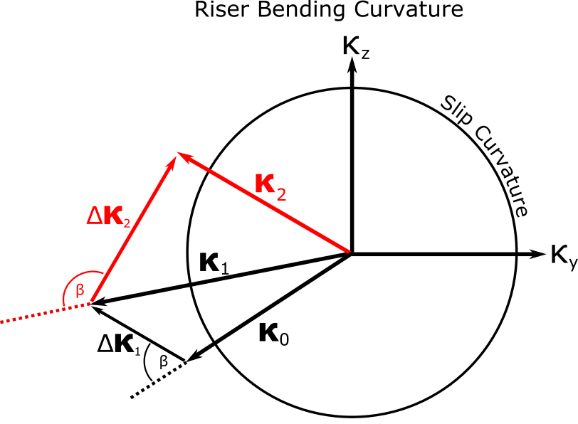
Curvature Reversal
A curvature reversal occurs between t = 1 and t = 2 because the curvature κ1 is outside the slip circle, and the angle between κ1 and Δκ2 is between 90º and 270º.
More details on how Flexcom models hysteretic bending is provided in Smith. et al., (2007).
•*BENDING HYSTERESIS is used to define hysteresis moment-curvature backbone curves for non-linear materials.
•*NO HYSTERESIS is used to suppress bending hysteresis effects.