Overview |
 
|
Overview |
|
Flexcom provides a comprehensive internal fluid modelling capability. Stationary internal fluids, uniform steady state internal fluid flow and multi-phase slug flow may all be modelled. If slugs are present in an analysis, they are displayed visually in the structural animation. This example considers the analysis of a rigid spool subjected to internal fluid and slug flow. The system is situated at a depth of 1500m, and consists of nine straight sections and eight 90-degree bends. Two contact surfaces are used to simulate the supports which help to reduce the possibility of seabed contact. The example consists of a static analysis, subject to gravity and buoyancy loads only, followed by a dynamic analysis subject to internal fluid and slug loading. The spool geometry is created using the Line Paths modelling feature.
If you are interested in further information regarding the effects of slug flow in rigid spools, please refer to the technical publication by Kavanagh et al., 2013.
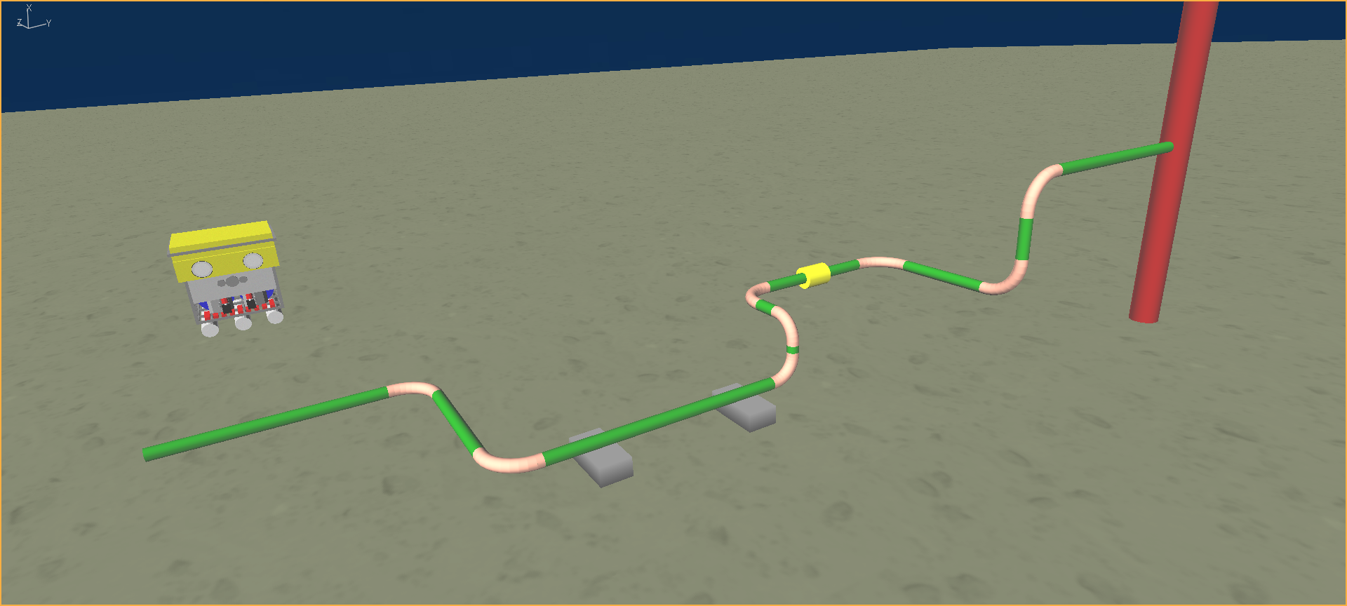
Spool Configuration
In the case of this model, the background fluid is gas, while the slug is oil. The flow direction is from left to right in the figure below. The slug colour (see dynamic animation) is slightly lighter at the tail end, denoting that the tail of slug has a lower density than the main body of the slug, as fluid density in the tail section decreases linearly from oil to gas. This approach is used to capture the effect of the oil and gas mixing together in a transition region at the back of the slug. The slug speed is also reduced slightly as it passes around each bend (3% decrease), leading to an overall decrease in flow velocity across the length of the slug. This aspect demonstrates the program’s ability to model time varying slugs which facilitate a more realistic slug flow definition than that of idealised flow of constant velocity.
An initial static analysis is performed in which the model is subjected to gravity and buoyancy loads only. This is followed by a dynamic restart analysis in which five successive oil slugs are passed through the spool. The time delay between each slug is such that a gap of three times the total slug length is maintained between each consecutive slug. Each slug is modelled as 25 metres long. To model the decaying density of the slug towards its tail end, two slugs of different density are used, with a time delay between them. The main body of the slug is 20m in length and this portion has uniform density. A secondary 5m slug is used to model the tail portion, whose density varies linearly from oil to gas.