Regular Wave Analyses |
 
|
Regular Wave Analyses |
|
For the purposes of this example, we will examine three regular wave load cases, corresponding to wave periods of 8s, 9s, and 10s, respectively, though in practice many more would also be examined. Combined with the near and far vessel offset case, this will result in 6 regular wave keyword files in total. Using the keyword parameterisation facility means that a single keyword file is all that is required to model each combination, and although the load case matrix is relatively small in this instance, the benefits are obvious. Refer to Keyword Parameterisation for further information on this feature.
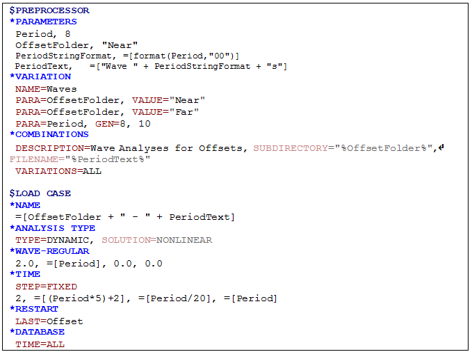
Create a new blank keyword file named Regular Wave.keyx, (or similar, depending on your naming convention) and include all the required data in this single base keyword file. The relevant input data is shown in the figure below. Note that that ![]() symbol indicates that the keyword data continues on the same line in the actual keyword file, even though it is necessary to show some data on a subsequent line here due to formatting constraints in this document.
symbol indicates that the keyword data continues on the same line in the actual keyword file, even though it is necessary to show some data on a subsequent line here due to formatting constraints in this document.
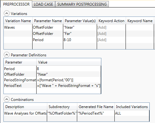
Regular Wave Load Case Variations
A number of points are noteworthy:
•The load case matrix is automatically determined by Flexcom. In this case, there are two parameters changing, 3 different wave periods combined with 2 different offset directories, resulting in a load case matrix totalling 6 separate dynamic analyses. Refer to the *PARAMETERS and *VARIATION keywords for further information on these data inputs.
•The names of the files are based on the period parameter, such as Wave 08s.keyx, and so on. All the newly created files are located in either the Near or the Far directory. Refer to the *COMBINATIONS keyword for further information on these data inputs.
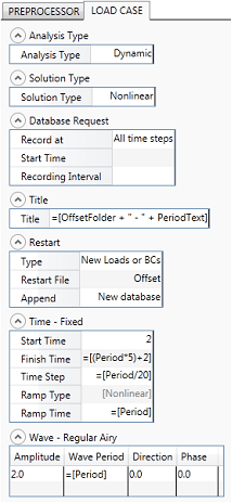
•Each dynamic analysis uses an appropriate regular wave period. A unit wave amplitude is used in all cases. Refer to the *WAVE-REGULAR keyword for further information on these data inputs.
•Appropriate time variables are computed based on the regular wave period. Each dynamic analysis runs for 5 wave periods, with the loads ramped on over the first wave period. A fixed time step equal to 1/20th of the regular wave period is used. Refer to the *TIME keyword for further information on these data inputs.
•The Analysis Type is set to Dynamic. Refer to the *ANALYSIS TYPE keyword for further information on these data inputs.
•Full database storage is requested for the regular wave analyses. Refer to the *DATABASE keyword for further information on these data inputs.
Flexcom provides a powerful facility for generating a Summary Output File. Here the maximum value, the minimum value, the range of values and the standard deviation of values is tabulated for a group of parameters you specify. The output is in a succinct format and could, for example, be pasted or inserted into a study report, or perhaps included as a report appendix. Refer to Summary Postprocessing for further information on this feature.
In this example, the postprocessing requests are specified before the analysis begins, via the standard output option. This option allows you to quickly request a summary of pertinent information, without the inconvenience of explicitly requesting specific outputs. For every element set referenced, Flexcom produces outputs of effective tension, resultant bending moment and von Mises stress for that set.

Summary Postprocessing Requests
Refer to the *STANDARD OUTPUT keyword for further information on these data inputs.
Once the specification of the regular wave data is complete, you should save the keyword file. Once you run the keyword file (Regular Wave.keyx, or similar, depending on your naming convention), Flexcom will automatically create a separate keyword file for you, corresponding to each combination of regular wave and preceding vessel offset directory. In order to perform the actual analyses themselves, you could run each analysis individually. However, a better approach is probably to invoke the Run Branch option from the vessel offset analyses.
Consistent with the concept of a highly project-focused integrated engineering environment introduced in Project Structure earlier, the keyword file interdependencies are readily evident at a glance in the File View. Specifically, at the top level lies the initial static analysis, which represents the starting point for all subsequent restart analyses. At the next level come the near and far vessel offset analyses, which restart directly from the initial static configuration. Next are the dynamic regular wave analyses, which are linked to the relevant offset analysis (i.e. near or far). So the entire keyword file hierarchy is clearly evident from the File View, as illustrated in the figure below.
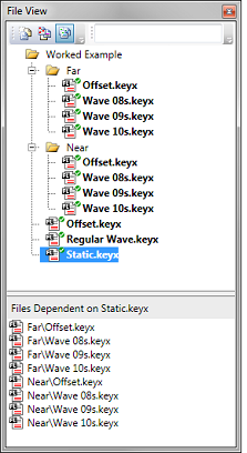
Keyword File Interdependencies
Unlike the database postprocessing performed for the initial static analysis, no plot files have been requested or created in this instance. Instead, each regular wave analysis produces a tabular summary file (with the extension SUM). The figure below shows some sample summary output, corresponding to the 8s regular wave analysis, for the near vessel offset case (this corresponds to the file Wave 08s.sum, or similar, depending on your naming convention). You can examine the other tabular summary files created for the other load cases at your convenience.

Sample Summary Output File