Model Building |
 
|
Model Building |
|
The model is largely created using lines. The majority of the central structure, including the upper and lower flex joints, the upper and lower frames, the outer pipe and the buoyancy tank, is modelled using a single line. A separate line is used to model the inner pipe. Another two lines are used to model the oil and gas jumpers. Finally, two further short lines are used to model the T-frame, which connects the jumpers to the central structure.
The lines functionality is a relatively recent addition to Flexcom, and essentially provides an automatic mesh creation facility whereby nodes, elements and cables can be generated quite easily. Using lines to build your model is a fundamentally different approach to working directly with nodes, elements and cables. While all the information is ultimately handled in the same fashion internally in the software, the use of lines expedites the model creation process considerably, as you need not concern yourself with individual node and element numbering. While the explicit numbering scheme (which was the only approach available in earlier versions of Flexcom) may appear obsolete by comparison, it is retained for complete generality, and also to maintain downward compatibility with previous versions. Refer to Lines for further information on this feature.
The majority of the central structure is modelled using a single line, running all the way from the seabed to the top of the buoyancy tank. This line includes the upper and lower flex joints, the upper and lower frames, the outer pipe and the buoyancy tank. For most vertical structures (e.g. drilling risers), a single line would be sufficient, but this model is slightly complicated by the fact that the riser is dual bore, so a separate line is required to model the inner pipe.
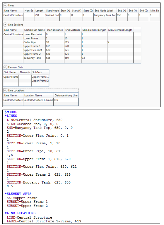
The first line is called Central Structure, and is assigned a length of 650m. Its start and end locations are called Seabed End {0m, 0m, 0m} and Buoyancy Tank Top {650m, 0m, 0m}. Obviously the structural properties of the structure vary along its length due to the different components, so it is necessary to define a number of subsections in terms of distances along the line. The subsections are called Lower Flex Joint (from 0m to 1m), Lower Frame (from 1m to 10m), Outer Pipe (from 10m to 615m), Upper Frame (from 615m to 620m, and from 621m to 625m), Upper Flex Joint (from 620m to 621m) and Buoyancy Tank (from 625m to 650m). In order to ensure that the automatic meshing algorithm positions a node on the upper frame at the correct elevation for connection to the T-frame, a line location is defined on the Central Structure called Central Structure T-Frame, at a distance of 619m along the line (i.e. 1m below the upper flex joint).
In terms of element lengths, it is desirable to model the upper and lower flex joints using a single element, so a suggested length of 1m is specified (which is equal to the joint length in both cases). A constant element length of 1m is also suggested for the lower and upper frames. Suggested minimum and maximum lengths of 1m and 5m, respectively, are suggested for the outer pipe. A constant element of 0.5m is suggested for the buoyancy tank. The definition of the Central Structure line in both the table and keyword editor is shown in the figure below.
Input data is organised into two main categories, model data and load case data. This distinction is reflected in both the table and keyword editors. Model data consists of information which must be specified in the very first of a series of consecutive analyses. This data is carried through to all subsequent restart analyses and may not be changed. This category naturally includes the finite element discretisation, structural and hydrodynamic properties, plus any other inputs which characterise the initial model configuration (e.g. initial vessel position, seabed properties, ocean depth etc.). Load case data may be entered in any analysis of a series of runs, and which may be subsequently altered in restart analyses. This category naturally includes environmental loading such as current and waves, boundary conditions, solution variables etc. There is a clear division between model and load case data in the keyword editor, via the $MODEL and $LOAD CASE sections in the keyword file. Similarly, in the table editor, the sections are split onto different tabs named MODEL and LOAD CASE. Before you enter the first keyword (i.e. *LINES, to define the central structure), you should include a $MODEL section entry. You can also add a MODEL section through the table editor by right-clicking on the table editor and selecting Add Section from the context menu.
The width of the columns in the table editor images that follow have been reduced due to formatting contraints in this document. Refer to the corresponding keyword editor excerpt to view the data values.
Central Structure Line
Refer to the *LINES, *LINE LOCATIONS and *ELEMENT SETS keywords for further information on these data inputs.
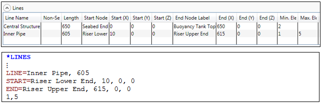
A second line (aptly named Inner Pipe) is defined to model the inner pipe, and is assigned a length of 605m. Its start and end locations are called Riser Lower End {10m, 0m, 0m} and Riser Upper End {615m, 0m, 0m}. As the inner pipe is composed of homogenous material with constant properties along its entire length, it is not necessary to define any subsections of the line. For consistency with the outer pipe, suggested minimum and maximum lengths of 1m and 5m, respectively, are also suggested for the inner pipe. The definition of the Inner Pipe line is shown in the figure below. Note that that symbol indicates that the following keyword data is supplementary to the existing data under the same keyword as shown previously.
Inner Pipe Line
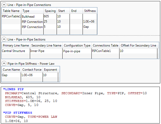
The upper and lower ends of the outer and inner pipes are rigidly connected using bulkheads (these are automatically modelled internally using equivalent nodes). The pipes are also connected at regular intervals (of 25m) using centralisers, and these are modelled using (linear) pipe-in-pipe connections of relatively large stiffness. Nonlinear “gap” connections are modelled at all nodal locations intermediate to the centralisers. The definition of the various pipe-in-pipe connections is shown in the figure below. Refer to Pipe-in-Pipe Configurations for further information on this feature.
Pipe-in-Pipe Connections
Refer to the *LINES PIP and *PIP STIFFNESS keywords for further information on these data inputs.
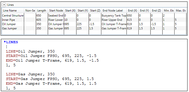
Two separate lines, Oil Jumper and Gas Jumper are used to model the jumpers, both having an assigned length of 350m. The start and end locations for the former are called Oil Jumper FPSO {695m, 225m, -1.5m} and Oil Jumper T-Frame {619m, 1.5m, -1.5m}, and Gas Jumper FPSO {695m, 225m, 1.5m} and Gas Jumper T-Frame {619m, 1.5m, 1.5m} for the latter. Suggested minimum and maximum lengths of 1m and 5m, respectively, are suggested for both jumpers. The definition of the Oil Jumper and Gas Jumper lines are shown in the figure below. Note that that ![]() symbol indicates that the following keyword data is supplementary to the existing data under the same keyword as shown previously.
symbol indicates that the following keyword data is supplementary to the existing data under the same keyword as shown previously.
Refer to the *LINES keyword for further information on these data inputs.
The T-Frame is modelled using two short lines. The first line, T-Frame-Top, is 3m long, and its start and end locations are T-Frame-1 {619m, 1.5m, -1.5m} and T-Frame-2 {619m, 1.5m, 1.5m}. The second line, T-Frame-Leg, is 1.5m long, and its start and end locations are T-Frame-4 {619m, 0m, 0m} and T-Frame-5 {619m, 1.5m, 0m}. In order to model this portion of the T-Frame using a single element, a suggested length of 1.5m is specified. The definition of the T-Frame lines is shown in the figure below. Note that that ![]() symbol indicates that the following keyword data is supplementary to the existing data under the same keyword as shown previously.
symbol indicates that the following keyword data is supplementary to the existing data under the same keyword as shown previously.

T-Frame Lines
Refer to the *LINES keyword for further information on these data inputs.
The intersection of the T-Frame is located at T-Frame-3, 1.5m along the line T-Frame-Top, as shown in the figure below.
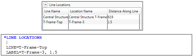
Line Locations on T-Frame
Refer to the *LINE LOCATIONS keyword for further information on these data inputs.
The top of the T-Frame is rigidly connected to its leg in reality, and the leg is rigidly connected to the central structure. Nodal equivalences are defined in the model in order to model these connections, as shown in the figure below. Refer to Connecting Lines for further information on this feature.

Nodal Equivalences on T-Frame
Refer to the *EQUIVALENT keyword for further information on these data inputs.
The top of the T-Frame is connected to the jumpers using free hinges in reality. Hinge elements are defined in the model in order to model these connections, as shown in the figure below. Refer to Hinges and Flex Joints for further information on this feature.
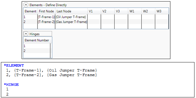
Hinge Elements
Refer to the *ELEMENT and *HINGE keywords for further information on these data inputs.
The Model View provides a “live” structure preview facility available during model building. It also allows you to view an animation of the structure response after an analysis has completed. The Model View allows you to rotate and pan the viewpoint, to zoom in and out, and has many other useful display features (feel free to experiment) such as node and element numbering, nodal coordinates, seabed topography, water surface profile etc. Once the geometric specification has been completed, the Model View provides a preview of the hybrid riser system, as shown in the figure below. Refer to Model View for further information on this feature.

Model View