Local (User-Defined) Axes |
 
|
Local (User-Defined) Axes |
|
In addition to the global and other pre-defined axes in Flexcom, the program does provide the option for you to define an arbitrary or ‘local’ system of axes (via *LOCAL AXIS SYSTEM). For example, rotational hydrodynamic coefficients for a point buoy may be defined with respect to a local axis system, or you may wish to apply boundary conditions in a local axis system. The local axes are defined by inputting, as components in the global axes, two of the three vectors defining the axes, namely the local x-axis and y-axis. These must be orthogonal, and provided they are, Flexcom works out the component of the local z-axis using the right-hand rule. For example, in the simplified specification below where the local axes simply represent a rotation of the global axes about global X, appropriate inputs for the local x-axis would be (1, 0, 0) while the local y-axis could be defined as (0, cos θ, sin θ).
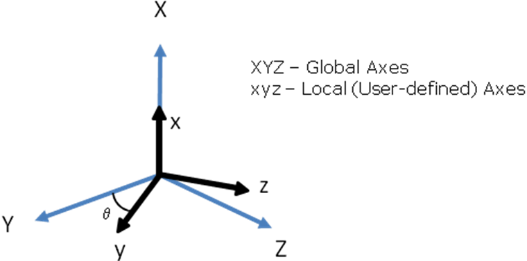
Local (User-Defined) Axes
When you create a local axis system via *LOCAL AXIS SYSTEM, this defines its initial orientation. The origin point and any associated motions depend on how the local axis system is used.
Once you reference a local axis system via *BOUNDARY, a dedicated local axis system is associated with the restrained node. This is a standalone entity, based on the user-defined axis definitions, coupled with a unique origin point whose initial position is set equal to the coordinates of the restrained node. It is possible that the same local axis system may be associated with more than one node, in which case Flexcom automatically creates several duplicate local axis systems, each with a different origin point. However recommended practice is to define more than one local axis system, with the same axis definitions, if you intend to constrain more than one node in the same local axis system. This affords you greater transparency should you wish to inspect the instantaneous position and orientation of the local axis system subsequently via *PRINT. Similar guidance applies to *POINT BUOY.
Local axis systems may be either fixed in space, or move with a node to which they are attached. For boundary nodes, the motion type is specified via *BOUNDARY, whereas for point buoys the axis system is always attached to the node.
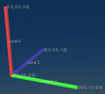
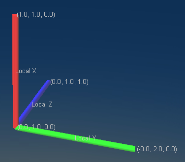
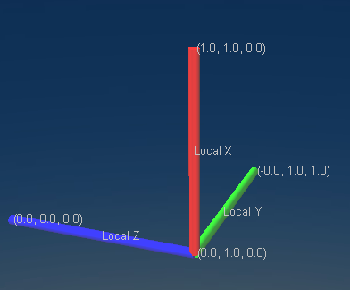
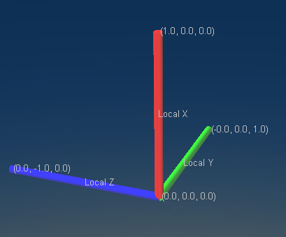
If you decide to apply boundary conditions with respect to a mobile local axis system, any translational displacements which you specify are applied with respect to the last updated state of the axis system, and may be built up cumulatively in different directions. For example, let's suppose you have a local axis system which is initially coincident with global, with the local origin at {0,0,0} and the local x, y and z axes aligned with the global X, Y and Z axes. You can add a triad of elements for visualisation purposes to facilitate the application of boundary conditions. If a +1m offset applied in the local y direction, this equates to +1m in global Y, and the origin moves to {0,1,0}. If a 90 degree rotation is applied about local x (= 90 degree rotation about global X), the origin remains at {0,1,0}, but the local y axis now aligns with the global Z axis. Then if a +1m offset applied in local z, this equates to -1m in global Y, so the origin moves back to {0,0,0}. So even though two positive displacement terms have been specified, the origin of the axis system has returned to its initial starting position. This simple test case shows how translational offsets may be applied consecutively in different directions.
|
|
|
|
Initial position |
+1m offset local y |
90 degree rotation about local x |
+1m offset local z |
Specification of non-zero boundary displacement terms with respect to mobile axis systems come with an inherent problem. When a displacement is applied to the node, the axis system naturally follows the node, creating a compound effect. In fact, the motion grows indefinitely as the displacement effect is never-ending. By default, the local axis system is updated at every solution iteration, but if there is any change to boundary displacement terms in the input specification, then the axis system is only updated at the end of the simulation.
•*BOUNDARY is used to define boundary conditions.
•*LOCAL AXIS SYSTEM is used to define local axis systems.
•*POINT BUOY is used to define point buoys and their associated hydrodynamic properties.
•*PRINT is used to request additional printed output to the main output file.