<< Click to Display Table of Contents >> Navigation:  Flexcom > Theory > Applied Loading > Wave Loading >
Jonswap Wave

Theory

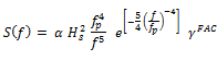
Hasselmann et al. (1973) developed a spectral formulation for developing seastates known as Jonswap (it originated during a Joint North Sea Wave Observation Project). It is essentially a modified version of the Pierson-Moskowitz spectrum, with some adjustments to align the spectrum with the measured North Sea data. The Jonswap spectrum is based on the following formulation:

       (1)

where:

                               (2)

and:

• is the Phillip’s constant

• is the spectral peak frequency

• is the peak period

• is the peakedness parameter

• is the spectral width parameter; = 0.07 for , = 0.09 for .

 

Specification Options

Flexcom offers a choice of formats for defining a Jonswap wave spectrum. The standard or default option is in terms of peak frequency fp, Phillips constant α, and spectrum peakedness parameter γ parameter, as per Equation 1 above. Alternatively you can define the data in terms of:

•Significant wave height Hs and mean zero up-crossing period Tz

•Hs and peak period Tp

•Hs, Tp and peakedness parameter γ

The first two alternative formats are different from the third in one respect. When you describe a spectrum in terms of Hs and Tz or Hs and Tp, then Flexcom uses special algorithms to select appropriate values for fp, α and γ. These algorithms are summarised shortly. Thereafter, Flexcom operates in exactly the same way as if the standard or default option had been invoked.

When the third (Hs, Tp and γ) format is invoked, a special algorithm (to be outline shortly) is used to calculate a value for α. The actual spectrum values are calculated using Goda’s approximation (Goda, 1979), as follows:

               (3)

Hs/Tz Format

For the Hs/Tz combination, the method adopted here is one due to Isherwood (1987), who publishes in his paper of 1987 a revised Jonswap spectrum parameterisation based on empirical data published by Houmb and Overvik (1976). This parameterisation will not be described in detail here; the interested reader is referred instead to the publications listed in the references. However the procedure is outlined here for completeness.

Isherwood first defines an equivalent wave steepness s as:

       (4)

where g is the gravitational constant. The value of γ is then found from:

       (5)

The value of α is next calculated from the relation:

               (6)

Finally the value of the peak frequency fp is found from:

                       (7)

Hs/Tp Format

For the Hs/Tp combination, Flexcom first categorises the seastate based on the value of the parameter (Tp /√ Hs). Values for γ and α are then calculated according to the table below; fp is simply 1/Tp.

Calculation of Jonswap Parameters

The numerical values in the table above are actually appropriate only for Hs in metres. If you specify a Jonswap spectrum in Hs/Tp format, Flexcom checks the value you specify for the gravitational constant g. If g is in the range 32 < g < 33, then the program assumes that your data is in Imperial units, and your value for Hs is converted internally to Metric before the table calculations. If your value for g is outside of this range, Hs is assumed to be in metres, and the table above's formulae are applied without modification.

Hs/Tp/γ  Format

For the Hs/Tp/γ combination, Flexcom uses this formula to calculate α.

               (8)

Equation 3 above is then used for the wave spectrum values.

Relevant Keywords

•*WAVE-JONSWAP is used to specify a JONSWAP random sea wave spectrum or spectra.