Spectrum Discretisation |
 
|
Spectrum Discretisation |
|
In a random sea analysis, Flexcom discretises the spectrum (or spectra) you specify into discrete harmonics, and uses these to generate a time history of random surface elevation using a Monte Carlo simulation technique. This provides the basic dynamic random excitation on the structure. The spectral discretisation procedure may be based on equal area increments of the wave spectrum or on a geometric progression of wave frequencies.
Note also that where an analysis contains two or more wave spectra, each spectrum is discretised and applied independently. In other words, Flexcom does not compile a single equivalent/composite spectrum before the discretisation process begins.
With an equal area discretisation, the random wave spectrum is discretised into component harmonics by dividing the area under the spectrum into segments of equal area. The area of each segment is the total area under the spectrum divided by a user-specified number of harmonics, and each area then defines a single harmonic in the discretisation. This procedure has the disadvantage that it leads to increasingly larger frequency increments at higher frequencies and so to a poor representation of higher harmonics in the wave elevation time series. There is a maximum frequency increment input which may be used to counteract this. If a particular segment requires a frequency increment greater than the specified maximum, the segment area is continuously halved until the required increment is less than the maximum. In general, this leads to a greater number of harmonics being returned by the discretisation than the requested number.
With a geometric progression discretisation, the wave spectrum is discretised into segments based on frequency increments that form a geometric progression. The procedure adopted is as follows. The total area under the wave spectrum up to a user-specified cut-off frequency is found, and the frequency that corresponds to the first 1% of the area under the wave spectrum is identified. Next, this frequency is multiplied by a constant factor to give the next frequency in the series. The area between these two frequencies is taken as the first discrete segment of the wave spectrum. The next frequency in the series is found by again multiplying the last frequency by the constant factor, and the area between these two frequencies is taken as the next discrete segment of the wave spectrum. This procedure is repeated until the frequency corresponding to the first 99% of the area under the wave spectrum is reached. The constant factor which multiplies successive frequencies is governed by a user input, as outlined in the below Equation.
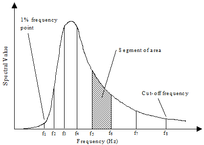
Geometric Progression Wave Spectrum Discretisation
The above figure shows an example of geometric progression wave spectrum discretisation. Each segment of area of the wave spectrum is defined by the frequencies at the start and end of the segment, fn and fn+1 as follows:
![]() (1)
(1)
where r is the user-specified geometric progression factor. Each segment of area defines a single harmonic in the discretisation, with the frequency of the harmonic for a particular segment given by:
![]() (2)
(2)
Flexcom uses a default value of 0.02 for the geometric progression factor, which is sufficient in most cases. The smaller the value used, the greater will be the number of harmonics in the resulting discretisation (and the longer will be the repeat time of the resulting wave elevation time series for time domain analysis). Note that the first figure above is illustrative only, generally a much larger number of harmonics should be produced by the wave spectrum discretisation.
Wave spectra may be defined using any of the following keywords:
•*WAVE-PIERSON-MOSKOWITZ is used to specify a Pierson-Moskowitz random sea wave spectrum or spectra.
•*WAVE-JONSWAP is used to specify a JONSWAP random sea wave spectrum or spectra.
•*WAVE-OCHI-HUBBLE is used to specify an Ochi-Hubble random sea wave spectrum or spectra.
•*WAVE-TORSETHAUGEN is used to specify a Torsethaugen random sea wave spectrum or spectra.
•*WAVE-TIME-HISTORY is used to specify a random seastate in terms of a time history of water surface elevation.
•*WAVE-USER-DEFINED is used to specify a User-Defined random sea wave spectrum or spectra.
Taking the Pierson-Moskowitz spectrum as an example, the FREQUENCY=AREA input is used to request equal area discretisation, while the FREQUENCY=GP input is used to request geometric progression discretisation.
•*PRINT is used to request additional printed output to the main output file. Specifically, the OUTPUT=WAVE DISCRETISATION option is used to request the wave discretisation details. When the option is invoked, the printed output might look like the following:
Sample Wave Discretisation Output
*** ADDITIONAL PRINTED OUTPUT ***
---------------------------------
Wave Discretisation Data:
Harmonic Omega Amplitude Phase Direction Wave Number Wave Length
(rad/s) (deg) (deg)
-------------------------------------------------------------------------------------
1 0.306371 0.176732 357.736 10.000 0.009930 632.746
2 0.328848 0.176732 348.678 10.000 0.011265 557.784
3 0.340204 0.176732 303.390 10.000 0.011990 524.040
4 0.348588 0.176732 76.948 10.000 0.012547 500.759
etc...
101 1.872890 0.088366 119.858 10.000 0.357566 17.572
102 2.159313 0.062484 239.289 10.000 0.475294 13.220
103 2.349804 0.062484 116.444 10.000 0.562852 11.163