Initial Static Analysis |
 
|
Initial Static Analysis |
|
The type of analysis to be performed must be specified in each $LOAD CASE section. In this example, a static analysis is firstly performed.
![]()
![]()
Analysis Type
Refer to *ANALYSIS TYPE for further information on these data inputs.
Flexcom presents a comprehensive range of options to fully describe the constraints which are applied to the finite element model. The various options include constant (time invariant constraints), vessel (to apply vessel motions), and several others including an arbitrary user-subroutine facility which provides for complete generality in terms of constraint application. The first two options are invoked in this example, with the base of the riser and vessel fixed in three of freedom. Note that the relevant node labels (i.e. Lower End and Upper End), are created automatically by the lines facility during model building, and referenced when defining boundary conditions. The specification of boundary condition data goes into the $LOAD CASE section of the file. Refer to Boundary Conditions for further information on this feature.
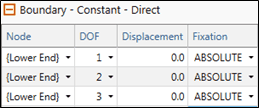
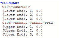
Initial Static Analysis - Boundary Conditions
Refer to *BOUNDARY for further information on these data inputs.
Flexcom provides a comprehensive internal fluid modelling capability. Stationary internal fluids, uniform steady state internal fluid flow and multi-phase slug flow may all be modelled. A stationary internal fluid in Flexcom is characterised by its mass density, pressure above hydrostatic and the level above the mudline to which it extends. In this example, the riser is filled with oil, as evident from its mass density. The level above mudline input is set equal to the riser elevation – Flexcom uses this input to determine whether elements are filled with fluid, and also to compute the hydrostatic pressure. Notice that internal fluid data is specified in a newly created $LOAD CASE section of the file. Refer to Internal Fluid for further information on this feature.
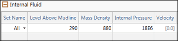
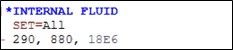
Internal Fluid
Refer to *INTERNAL FLUID for further information on these data inputs.
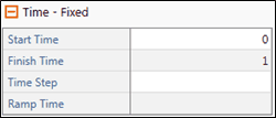
Naturally, all time domain analyses require the specification of time variables. Since a static analysis is one which considers time invariant loading and structure response, time variables are effectively meaningless in this context, however it is required to specify time variables for a static analysis in Flexcom. This is purely a consequence of the historical evolution of the software.
An initial static analysis is typically run from t=0 to t=1 second using a single fixed time step, and this standard approach is adopted for this example, as shown below. Refer to Time Variables in Static Analysis for further information on this feature.
![]()
Initial Static Analysis Time Variables
Refer to *TIME for further information on these data inputs
Database Postprocessing is the most powerful and widely used postprocessing facility in Flexcom. The database files provide a very detailed picture of the structure response. For large models, or long simulations with a large number of database outputs, the database files can become quite large. However, this is not a concern for static analyses, or indeed the dynamic analysis studied in this example. Refer to Database Postprocessing for further information on this feature.
In this example, the postprocessing requests are specified before the analysis begins, via the standard output option. This option allows you to quickly request a summary of pertinent information, without the inconvenience of explicitly requesting specific outputs. For every element set referenced, Flexcom produces outputs of effective tension, resultant bending moment and von Mises stress for that set.
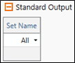
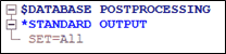
Database Postprocessing Requests
Refer to *STANDARD OUTPUT for further information on these data inputs.
Specification of the model geometry, structural and hydrodynamic properties, environment and loading data, vessel and RAO data, boundary conditions and solution parameters is now complete, so you should save the keyword file and run the analysis.
When a run is in progress, you can monitor its status via the Analysis Status View. The progress bar is naturally most beneficial for longer dynamic analyses (e.g. where it provides an approximate estimate of remaining CPU time), and sample progress information is shown below.
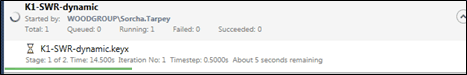
Analysis Progress Indicator
Another useful feature in the File View is that the program provides an indication of the status of the analysis. When the run has finished, the icon associated with the keyword file changes to ![]() , indicating that the analysis has completed successfully. You may have noticed the icon next to the keyword file name was previously
, indicating that the analysis has completed successfully. You may have noticed the icon next to the keyword file name was previously ![]() , indicating the analysis had not yet been run. As the computation time for the static analysis is relatively short, you probably won’t have noticed that the icon briefly changed to
, indicating the analysis had not yet been run. As the computation time for the static analysis is relatively short, you probably won’t have noticed that the icon briefly changed to ![]() , indicating that the analysis was currently in progress
, indicating that the analysis was currently in progress
You can view the analysis results using the Plotting facility. Plot files have the file extension .MPLT (an abbreviation of Mcs PLoT). The figure below shows the static effective tension distribution in the riser (this corresponds to the file K1-SWR-static.S1.mplt, or similar, depending on your naming convention). You can examine the other plots created for the static analysis at your convenience. Refer to Plotting for further information on this feature

Static Effective Tension
Similar results can obtained using the Excel Add-in, as shown below. This plot was quickly created using the Force Snapshot template from the Flexcom ribbon control.

Static Effective Tension