Dynamic Analysis |
 
|
Dynamic Analysis |
|
The presence of waves, whether regular or random, requires you to specify a dynamic analysis. As Flexcom has traditionally been a time domain analysis tool, existing users may instinctively associate “dynamic analysis” with “time domain”. The vast majority of time domain analyses are non-linear, and this option is selected by default. Refer to Time Domain Analysis for further information on this feature.
Create a new blank keyword file which uses the metric unit system and name it K1-SWR-dynamic.keyx, (or similar, depending on your naming convention).
You may define constant parameters within a keyword file, and reference these parameters when defining input variables. If you choose to define any such parameter, their definitions must appear at the beginning of the keyword file, under the $PREPROCESSOR section. When referencing a parameter, the variable definition must be preceded by the characters =[ and followed by the ] character. Specifically the variable definition will appear in the format =[Parameter], rather than just having an explicitly specified value. Refer to Parameters for further information on this feature.
For the purposes of this example, we will examine a regular wave load case, corresponding to wave periods of 10s, though in practice many more waves would also be examined. A new parameter call Period is defined, and assigned a value of 10 seconds as shown below.
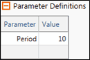

Period Parameter
Refer to *PARAMETERS for further information on these data inputs.
The type of analysis to be performed must be specified in each $LOAD CASE section. In this example, a dynamic analysis is required.

![]()
Analysis Type
Refer to *ANALYSIS TYPE for further information on these data inputs.
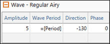
In this example, a regular wave of period of 10 seconds and amplitude of 5 meters is created. The wave direction is measured in degrees anti-clockwise from the global Y-direction and all waves in Flexcom emanate from the origin. The default direction is 0°, however for this example the direction is set at -130° aligned with the local vessel surge axis. Refer to Regular Airy Wave for further information on this feature.
![]()
Wave Properties
Refer to *WAVE-REGULAR for further information on these data inputs.
In a variable step analysis, the choice of time step magnitude is made by the program based on a number of criteria. The time step is continuously monitored and varied as appropriate by the program within user-specified limits, to ensure a stable and convergent solution. A variable step is typically used in analyses where the structural response varies significantly during the course of the simulation. Appropriate time variables are computed based on the regular wave period. The dynamic analysis runs for 5 wave periods, with the loads ramped on over the first wave period. A fixed time step equal to 5% of the wave period is used. Refer to Variable Time Stepping and Choice of Time Step for further information on these features.
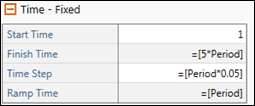
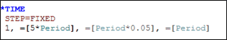
Dynamic Analysis Time Stepping
Refer to *TIME for further information on these data inputs.
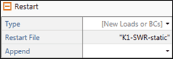
The Restart facility allows us to specify that a particular analysis is to be restarted from a previous run, to build up to the full dynamic solution in stages. In a restart, the structure configuration at the end of the preceding analysis becomes the starting configuration for the restart. Refer to Restart Analysis for further information on this feature.
In this case we want to restart the present run from the K1-SWR-static file.
![]()
Restart Analysis
Refer to *RESTART for further information on these data inputs.
For this analysis the Statistics output category is used. Options are provided for plotting statistics of motions and forces for specified element sets or the whole structure. Outputs include maximum/minimum envelopes, mean values, standard deviations and extreme values. Refer to Database Postprocessing for further information on this feature.
In this example a plot of the maximum/minimum envelopes of effective tension and bending moment is requested. Variable values are assigned to different force statistics for ease of use. In this case the variable value of 7 corresponds to effective tension and the value of 8 corresponds to bending moment. The statistic output feature is calculated over the last two periods in this example. Flexcom excludes any values before this time.
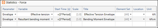
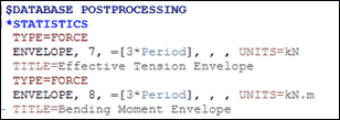
Database Postprocessing Requests
Refer to *STATISTICS for further information on these data inputs.
Once the specification of the dynamic data is complete, you should save the keyword file and run the analysis.
When a run is in progress, you can monitor its status via the Analysis Status area. The progress bar is naturally most beneficial for longer dynamic analyses (e.g. where it provides an approximate estimate of remaining CPU time), and sample progress information is shown below.

Another useful feature in the File View is that the program provides an indication of the status of the analysis. When the run has finished, the icon associated with the keyword file changes to![]() , indicating that the analysis has completed successfully. You may have noticed the icon next to the keyword file name was previously
, indicating that the analysis has completed successfully. You may have noticed the icon next to the keyword file name was previously ![]() , indicating the analysis had not yet been run. As the computation time for the static analysis is relatively short, you probably won’t have noticed that the icon briefly changed to
, indicating the analysis had not yet been run. As the computation time for the static analysis is relatively short, you probably won’t have noticed that the icon briefly changed to![]() , indicating that the analysis was currently in progress
, indicating that the analysis was currently in progress
You can view the analysis results using the Plotting facility. Plot files have the file extension .MPLT (an abbreviation of Mcs PLoT). The plot below shows the static effective tension distribution in the riser (this corresponds to the file K1-SWR-dynamic.D1.mplt, or similar, depending on your naming convention). You can examine the other plots created for the static analysis at your convenience. Refer to Plotting for further information on this feature
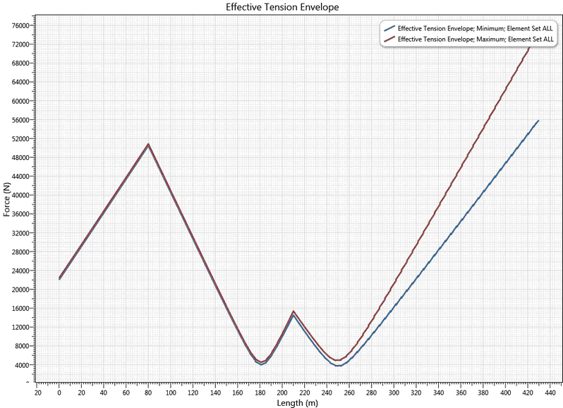
Dynamic Analysis - Effective Tension Envelope