Dynamic Analysis |
 
|
Dynamic Analysis |
|
Results from the dynamic analyses are presented in the figures below; each plot compares results from the time and frequency domain analyses. In this example, von Mises stress and effective tension are the critical parameters. The seabed touchdown and hang-off regions are the key locations.
The Dynamic Tensions figure below shows a plot of standard deviation of effective tension from the three analyses. Note that in this plot ‘Seastate 1’ refers to the 1m Hs, ‘Seastate 2’ to the 2m Hs, and ‘Seastate 3’ to the 3m Hs. Excellent agreement is observed between time and frequency domain analyses for the lowest Hs, the agreement is still good for the 2m case, while for the 3m case the agreement is less good but still reasonable. This is discussed in more detail presently.
The Dynamic von Mises Stresses figure below shows a plot of standard deviation of von Mises stress. There are noticeable peaks, located approximately 315m along the riser, which are typical of this type of simulation. These peaks naturally correspond to the SCR touchdown region. A second, lesser peak can be observed at the riser hang-off.
Time and frequency domain results are in close agreement everywhere except in the touchdown region. The almost exact agreement at the vessel connection is particularly noteworthy. The touchdown region stresses are more closely examined in the Dynamic von Mises Stresses (Detail) figure below, which shows a detail from Dynamic von Mises Stresses figure below. Here again it is clear than the time and frequency approaches give almost identical results for the 1m case, are in reasonable agreement for the 2m, but differ significantly for the highest Hs.
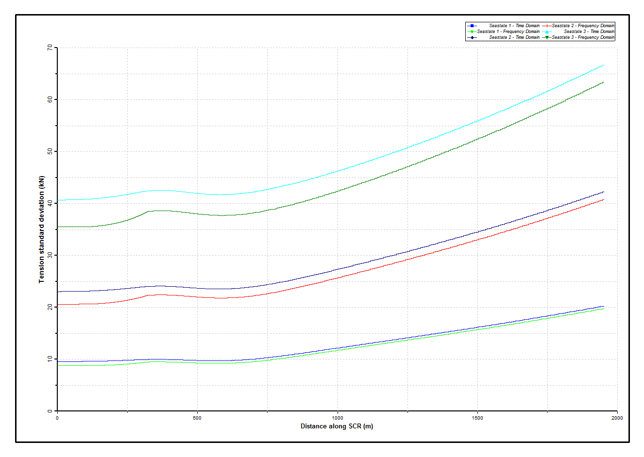
Dynamic Tensions
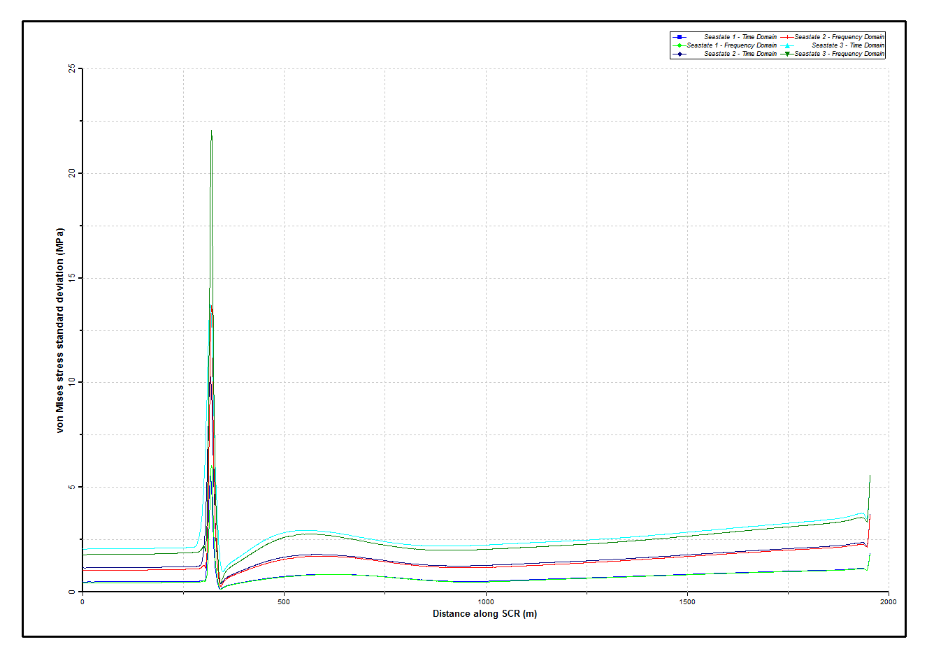
Dynamic von Mises Stresses
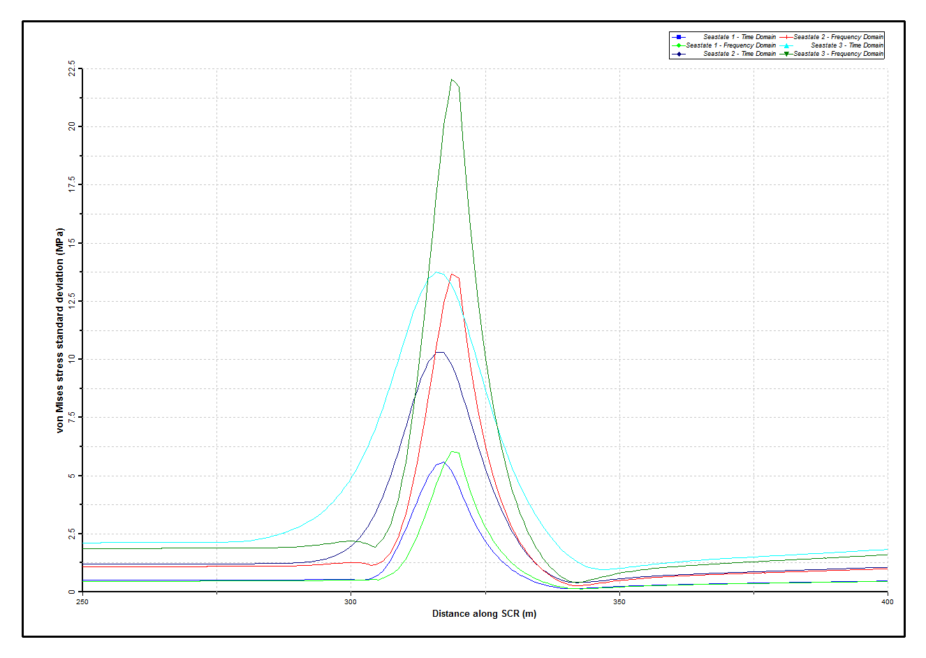
Dynamic von Mises Stresses (Detail)
Differences between the time and frequency domain results can be attributed to the fact that nodes that are on the seabed in the static configuration remain on the seabed throughout the frequency domain analysis. In the time domain on the other hand the changing nature of the riser/seabed interaction is accurately modelled. This means that dynamic stress variations are spread over a greater length of riser in the time domain, with a consequent reduction in the peak values – compare for example the differing extents of the touchdown region in the two graphs for Seastate 3 in the Dynamic von Mises Stresses (Detail) figure above. Obviously this effect is more pronounced in the higher seastates because the vessel motions are larger and the riser/seabed interaction more significant. It is worth pointing out that the SCR dynamic analyses in the frequency domain takes only a couple of minutes on a standard PC, compared to about an hour for the corresponding time domain runs.