Results |
 
|
Results |
|
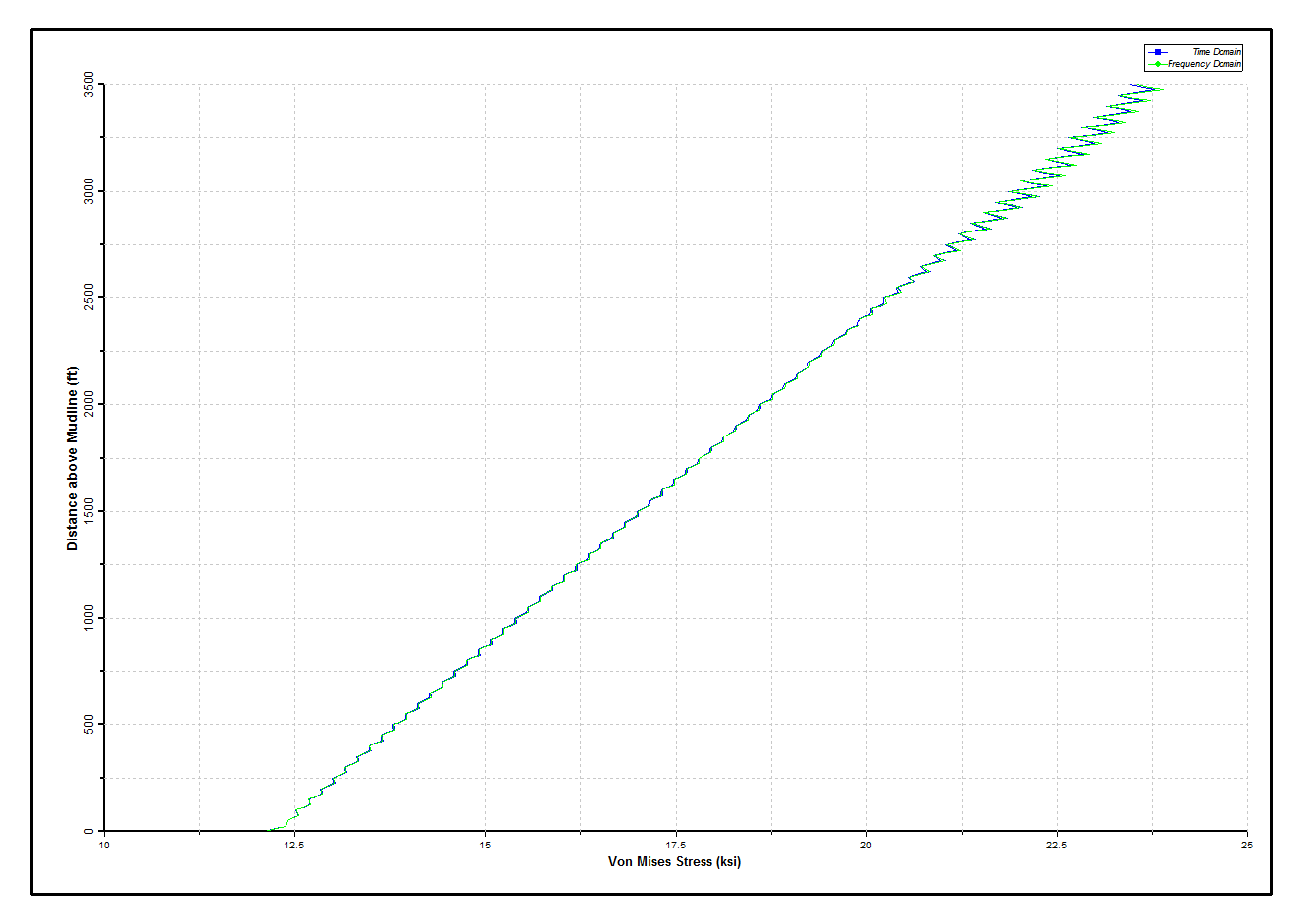
Dynamic results from both time domain and frequency domain analyses are presented below in terms of envelopes of effective tension and von Mises stress for the three sections. Results in all cases are plotted for elements up to 100 ft below the Spar keel; above this point unrealistically high stresses could be expected due to the crude nature of the Spar/riser interaction model used here. In the case of the tubing, results are presented for elements above the mudline only.
The Dynamic Tensions in Production Tubing figure and Dynamic Stresses in Production Tubing figure below show the results for the production tubing. Assuming the steel in the riser is Grade 80, the stresses are everywhere below allowable. Overall the dynamic variation is small, as might be expected with 8,000 ft of tubing below the mudline included in the model. Next, the corresponding plots for the inner riser are presented in the Dynamic Tensions in Inner Riser figure and Dynamic Stresses in Inner Riser figure below. The somewhat “jagged” plot is due to the variation in bending moment caused by the two different and alternating pipe-in-pipe connection types. Finally, the outer riser results are shown in the Dynamic Tensions in Outer Riser figure and the Dynamic Stresses in Outer Riser figure below. The agreement of results obtained from the time domain and frequency domain analyses is shown to be excellent.
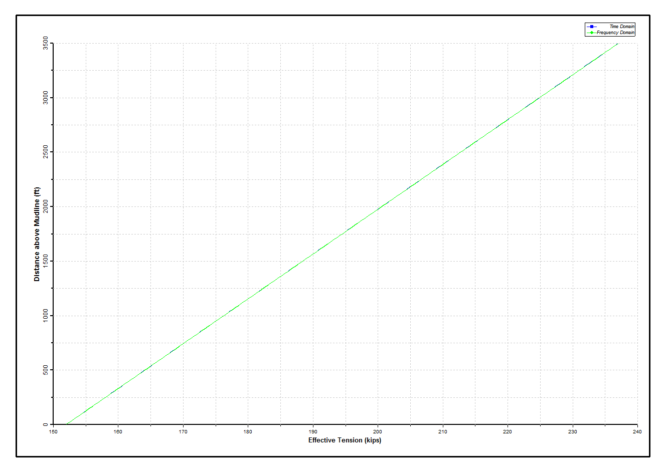
Dynamic Tensions in Production Tubing
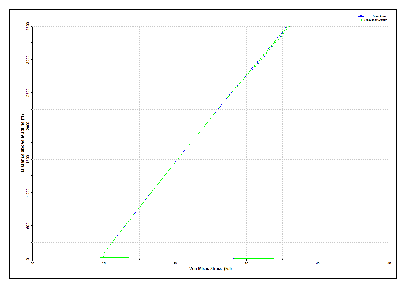
Dynamic Stresses in Production Tubing
Dynamic Tensions in Inner Riser
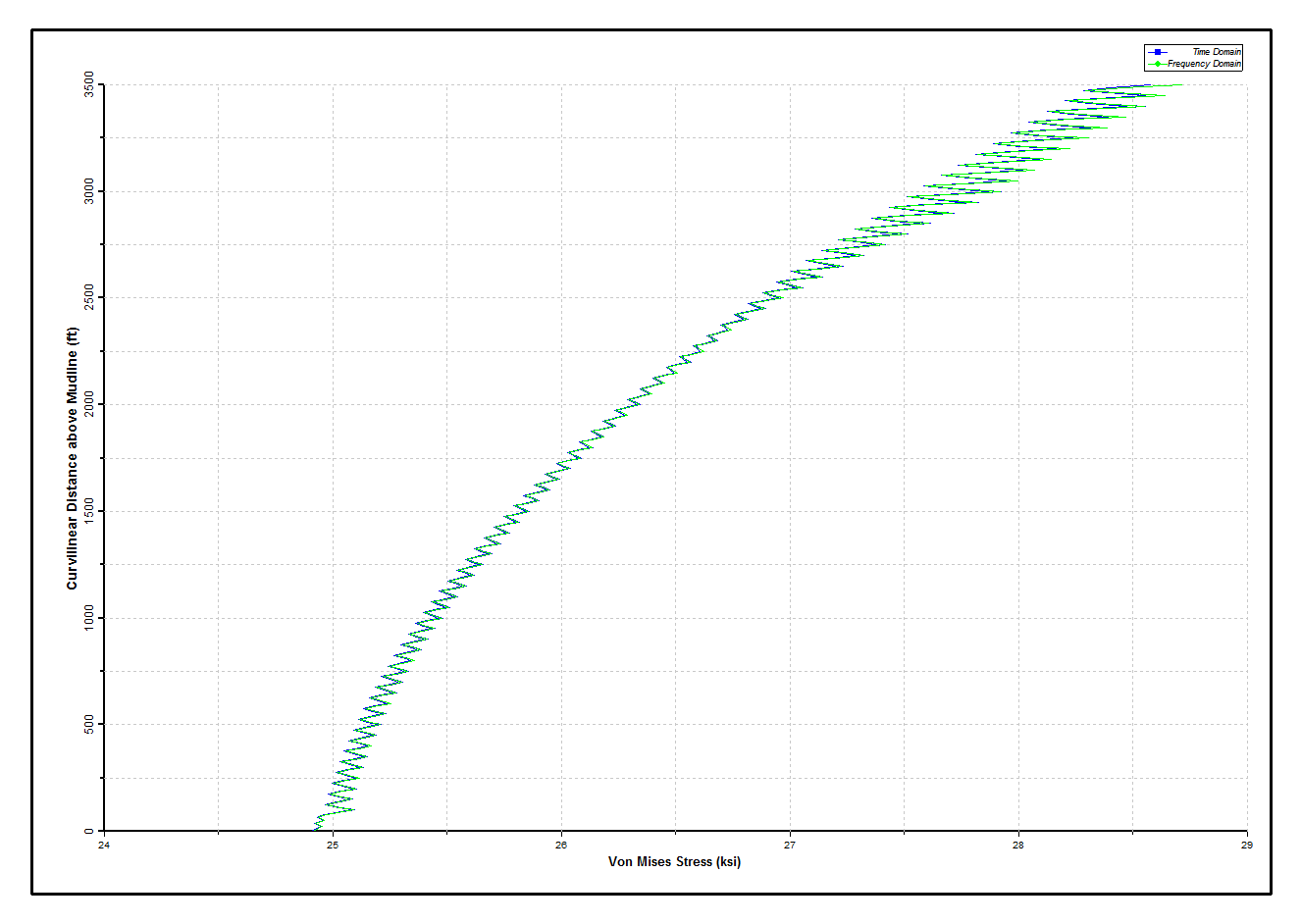
Dynamic Stresses in Inner Riser
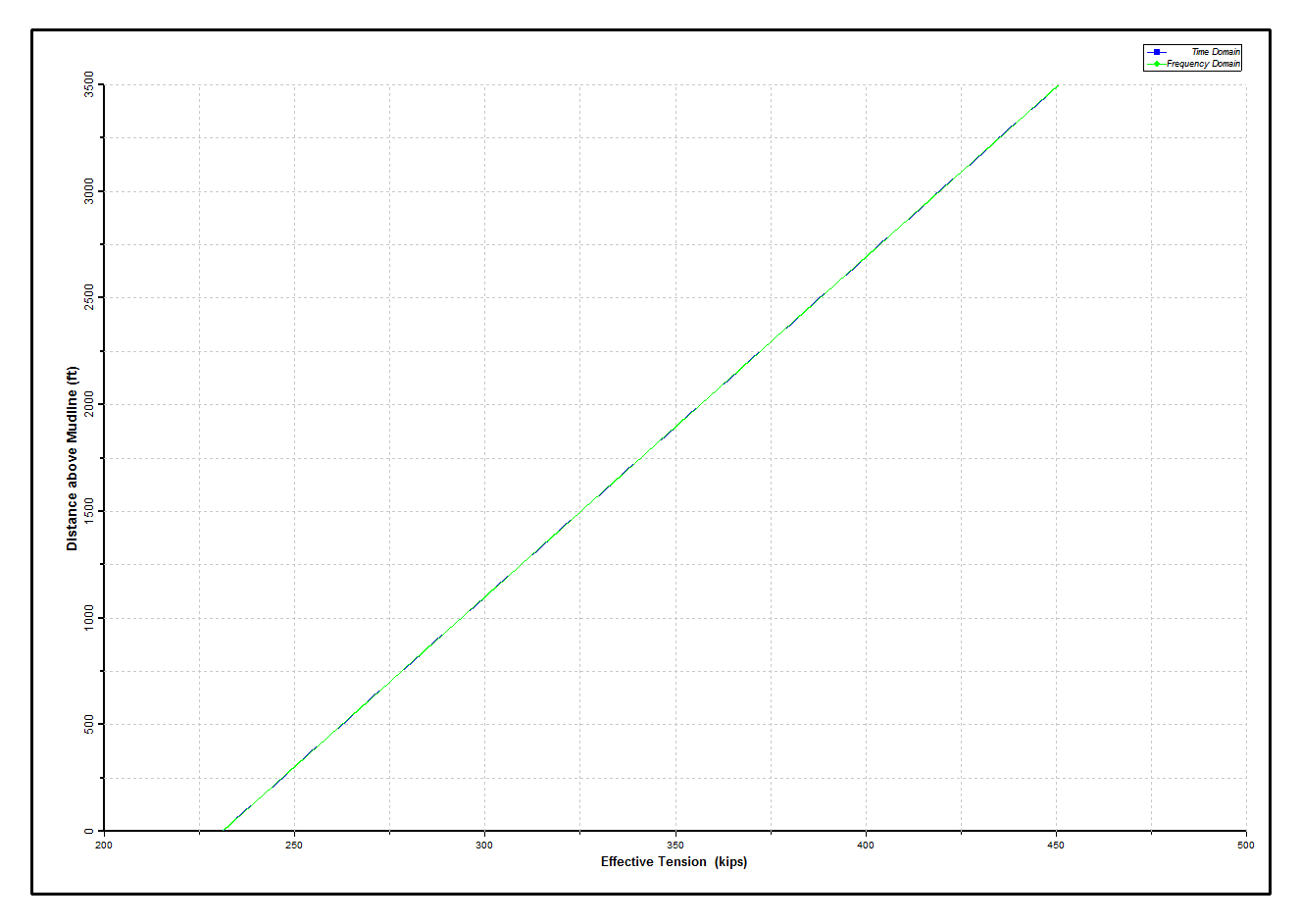
Dynamic Tensions in Outer Riser
Dynamic Stresses in Outer Riser
Results from the modal analysis are summarised below. It is clear from the table that the bending modes occur in identical pairs at each modal frequency, which is expected behaviour for a top-tensioned riser. This data is subsequently passed to Shear7 via the MDS file.
*** Summary of Results ***
--------------------------
---------------------------------------------------------------------------------------------------------------------------
Max Y- Max Z- Max
Max Bending Bending Combined
Eigenpair Eigenvalue Period Type Curvature Stress Stress Stress
(s) (1/ft) (lbf/ft^2) (lbf/ft^2) (lbf/ft^2)
---------------------------------------------------------------------------------------------------------------------------
1 0.0927 20.6340 Bending 0.3894E-04 0.0000E+00 0.5823E+05 0.5823E+05
2 0.0932 20.5799 Unknown 0.0000E+00 0.0000E+00 0.0000E+00 0.0000E+00
3 0.3714 10.3103 Bending 0.7561E-04 0.0000E+00 0.1131E+06 -0.1131E+06
4 0.3733 10.2833 Unknown 0.0000E+00 0.0000E+00 0.0000E+00 0.0000E+00
5 0.8361 6.8715 Bending 0.1123E-03 0.0000E+00 0.1681E+06 0.1681E+06
6 0.8405 6.8534 Unknown 0.0000E+00 0.0000E+00 0.0000E+00 0.0000E+00
7 1.4874 5.1519 Bending 0.1489E-03 0.0000E+00 0.2232E+06 -0.2232E+06
8 1.4952 5.1384 Unknown 0.0000E+00 0.0000E+00 0.0000E+00 0.0000E+00
9 2.3258 4.1200 Bending 0.1854E-03 0.0000E+00 0.2783E+06 0.2783E+06
10 2.3381 4.1091 Unknown 0.0000E+00 0.0000E+00 0.0000E+00 0.0000E+00
11 3.3523 3.4317 Bending 0.2220E-03 0.0000E+00 0.3341E+06 -0.3341E+06
12 3.3700 3.4227 Unknown 0.0000E+00 0.0000E+00 0.0000E+00 0.0000E+00
13 4.5677 2.9399 Bending 0.2584E-03 0.0000E+00 0.3896E+06 0.3896E+06
14 4.5920 2.9321 Unknown 0.0000E+00 0.0000E+00 0.0000E+00 0.0000E+00
15 5.9734 2.5708 Bending 0.2953E-03 0.0000E+00 0.4465E+06 -0.4465E+06
16 6.0052 2.5640 Unknown 0.0000E+00 0.0000E+00 0.0000E+00 0.0000E+00
17 7.5706 2.2836 Bending 0.3312E-03 0.0000E+00 0.5022E+06 0.5022E+06
18 7.6111 2.2775 Unknown 0.0000E+00 0.0000E+00 0.0000E+00 0.0000E+00
19 9.3609 2.0536 Bending 0.3705E-03 0.0000E+00 0.5637E+06 -0.5637E+06
20 9.4112 2.0481 Unknown 0.0000E+00 0.0000E+00 0.0000E+00 0.0000E+00
21 11.3461 1.8653 Bending 0.4057E-03 0.0000E+00 0.6197E+06 0.6197E+06
22 11.4073 1.8603 Unknown 0.0000E+00 0.0000E+00 0.0000E+00 0.0000E+00
23 13.5280 1.7083 Bending 0.4420E-03 0.0000E+00 0.6779E+06 -0.6779E+06
24 13.6013 1.7037 Unknown 0.0000E+00 0.0000E+00 0.0000E+00 0.0000E+00
25 15.4122 1.6005 Torsional 0.0000E+00 0.0000E+00 0.0000E+00 0.0000E+00
From the perspective of a VIV-induced fatigue assessment of the inner riser, the results of interest from Shear include:
•Numbers of the excited modes (taken from section "2.2.1 Results of the Mode Interaction Analysis")
•Modal time share probabilities (taken from section "2.2.1 Results of the Mode Interaction Analysis")
•Modal frequencies (taken from section "9. Modal damping ratio "zeta", modal mass, and modal frequency for the mainly excited modes")
•Modal amplitudes (taken from "11. Modal Displacement Amplitude")
Relevant extracts from the Shear7 output file are reproduced here in order to help you to familiarise yourself with the various data outputs (assuming you are not an experienced user of Shear7).
Shear7 Output File Extracts
2.2.1 Results of the Mode Interaction Analysis:
Based on the non-zero power-in lengths and the power cutoff value of: 0.05
the number of modes above cutoff is: 5
These modes are: Time Share Excitation Dominant Mode
Probabilities: Zone # Amplitude:
5 0.6776 1 0.1000E+01
6 0.1154 1 0.9805E+00
10 0.0529 1 0.5515E+00
11 0.0731 1 0.5394E+00
12 0.0811 1 0.5237E+00
-------- --------
Cumulative sum: 1.0000 Primary zone amplitude limit: 0.3000
Lowest And Highest Excited Mode Number
Nmmin= 5 Nmmax= 12
9. Modal damping ratio "zeta", modal mass,
and modal frequency for the mainly excited modes.
mode no. damping ratio modal mass(slug) frequency (Hz)
-------------------------------------------------------
5 0.15389 2568.612 0.24273
6 0.10722 2565.540 0.29140
10 0.05928 2557.277 0.48695
11 0.05150 2535.415 0.53610
12 0.04567 2588.692 0.58537
11. Modal Displacement Amplitude
Mode No. Amplitude (ft or m)
---------------------------------
5 0.38520
6 0.38644
10 0.08868
11 0.09435
12 0.08762
The solution database produced by Modes contains information on all modes (whether bending, axial, torsional or mixed modes), while the Shear7 output relates specifically to pure bending modes. In order to extract the relevant mode shapes from Modes, the relevant mode number are obtained from the Modal Solution Summary table, using the Shear7 mode number as an index in the table. For example, the first VIV mode identified by Shear7 is Mode No.5, and this corresponds to Mode No.9 in the output from Modes. All 5 mode shapes of interest overlaid in a single plot are shown below. Although not an issue in this case, it is advisable to examine the various mode shapes to verify that they represent pure bending modes (viewing two separate planes side-by-side in the Model View is quite helpful in this respect) and reduce the possibility of mixed modes being included.

Mode Shapes
Results from the fatigue analysis are summarised below. The fatigue life predicted by the Rainflow Cycle Counting method is just over 8 years, so fatigue is clearly an issue for the riser system as it currently stands. The engineering design team would probably look into VIV suppression mechanisms such as strakes or fairings. It should be noted that this is a highly simplified example which is provided for illustrative purposes only. Only one current profile is considered in Shear7, whereas in reality a range of current profiles would be simulated to cover the range of loading conditions likely to be experienced by the riser system. Your attention is also drawn to the other Model Simplifications listed earlier.
Results Summary
===============
Damage Calculated Directly from Time History
Maximum predicted damage : .14738E+00
Corresponding fatigue life: 6.79 years
Occurring at element : 1145
Stress point : 1
Damage Calculated from Stress Spectrum
Maximum predicted damage : .21535E+00
Corresponding fatigue life: 4.64 years
Occurring at element : 1145
Stress point : 1
Damage Calculated from Rainflow Counting
Maximum predicted damage : .12238E+00
Corresponding fatigue life: 8.17 years
Occurring at element : 1145
Stress point : 1