Results |
 
|
Results |
|
The static riser solution is shown in the Static Effective Tension Distribution figure to Dynamic Effective Tension Envelope Base Case figures below, which plot respectively the static structure configuration and the static distributions of tension and curvature in the riser. The Static Resultant Curvature Distribution figure shows that in its mean static position the riser is everywhere in effective tension. The large peak in curvature at the fixed vessel hangoff, where the bend stiffener is located, is also noteworthy.
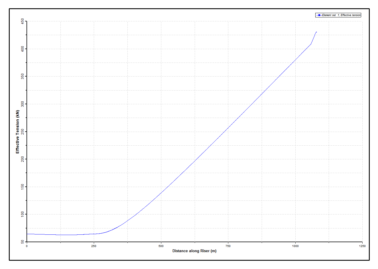
Static Effective Tension Distribution
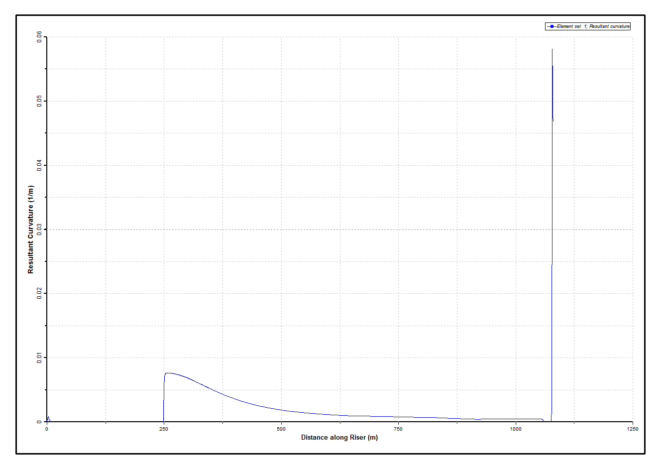
Static Resultant Curvature Distribution
The Dynamic Effective Tension Envelope Base Case figure below presents the envelope of effective tension from the base case dynamic analysis, with the 0.01s time-step.
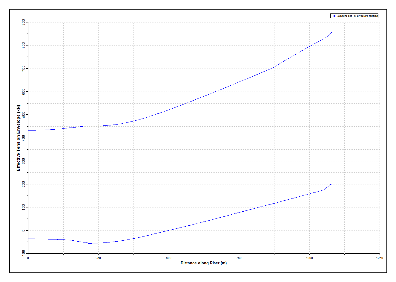
Dynamic Effective Tension Envelope Base Case
Clearly effective compression is predicted in the riser on the seabed. The minimum predicted value is approximately (-)52kN. Note that in the model used here, element lengths on the seabed vary between 0.5m and 3m. For an element of length 3m and bending stiffness 57.82kNm2, the critical Euler buckling load is ~63kN. For an element of length 0.5m, it is ~2280kN. So the Euler buckling load is not exceeded in any individual element here, as per the findings of McCann et al., (2003).
The Localised Buckling in Touchdown Zone figure below illustrates the configuration in the touchdown zone at a sample solution time during which the riser is in compression. The presence of localised buckling is clearly evident.

Localised Buckling in Touchdown Zone
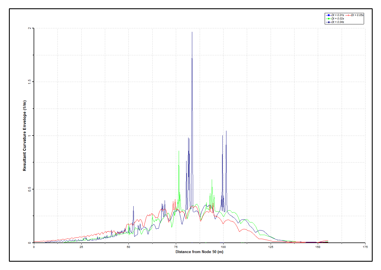
The remaining figures show the effect of time-step size on curvature statistics. The Curvature Envelopes – Sensitivity to Time-Step figure shows max/min envelopes for the four time-step values used in this study, while the Curvature Deviations – Sensitivity to Time-Step figure plots the corresponding curvature standard deviations. A significant variation is observed in the Curvature Envelopes – Sensitivity to Time-Step figure with changing time-step. This is due to differences in the post-buckling behaviour of the riser. McCann et al show that the way in which buckling progresses is strongly influenced by the deformed position of the riser as buckling is initiated (McCann et al., 2003). So slight differences in deformed position between analyses with different time-steps lead to quite different behaviour thereafter.
On the other hand the Curvature Deviations – Sensitivity to Time-Step figure shows that standard deviations tend to be more uniform than the corresponding curvature distribution, even for the analysis with the large time-step (0.04s), the results from which in the Curvature Envelopes – Sensitivity to Time-Step figure appear untrustworthy. McCann et al report a similar conclusion from a sensitivity study based on element length. On that basis, they conclude that using a deterministic approach in selecting the most onerous curvature condition can lead to large errors, and that the use of a statistical extrapolation based on standard deviation provides a more robust method of deriving maximum curvature (McCann et al., 2003).
Curvature Envelopes – Sensitivity to Time-Step
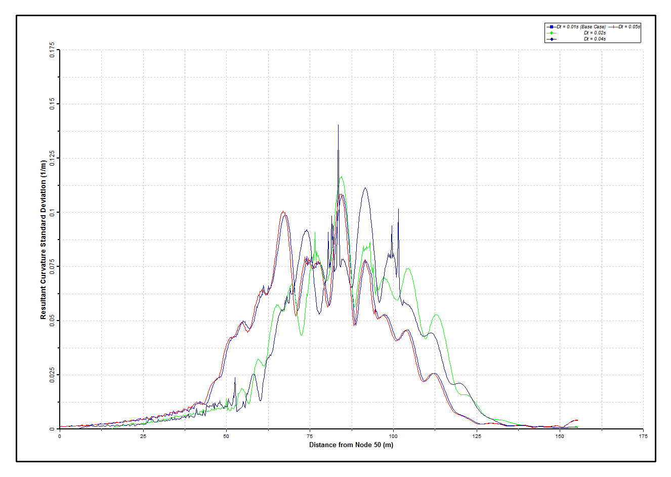
Curvature Deviations – Sensitivity to Time-Step