Operation |
 
|
Operation |
|
Typically, the uppermost P-y curve data is specified at some level below the mudline, but for complete generality, it is possible to specify P-y curve data at negative depths (i.e. at levels above the mudline). For example, the figure below shows a concrete casing extending above the mudline.
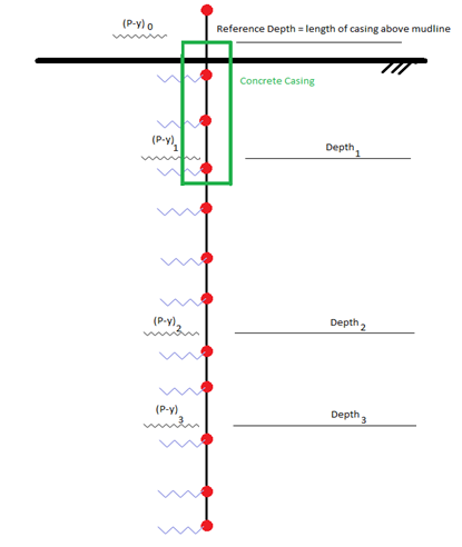
P-y Definition Schematic
A reference depth, d0, is defined as the depth of the uppermost P-y curve definition, or zero (representing the depth of the mud line), whichever is the higher elevation. Nodes beneath this reference depth are included in the soil resistance model.
Note also that you have the option to apply P-y curves to specific element sets. This allows you to cater for complex models (e.g. pipe-in-pipe configurations), or multiple risers located in different regions with dissimilar soil resistance characteristics. If no such sets are specified, all nodes below the reference depth are considered for soil resistance by default.
The resistance at a depth d between Depth1 d1 and Depth2 d2 is for a given lateral displacement y calculated as follows. Firstly the slopes of the P-y curve corresponding d1 and d2 are calculated from y: call them S1 and S2 respectively. An average slope S(y) is then calculated at d by linear interpolation using:
![]() (1)
(1)
where w1 and w2 are weighting functions defined by:

![]() (2)
(2)
The resistance P(y) is then given by:
![]() (3)
(3)
The resistance at a depth between the reference depth and the smallest depth for which a specification exists, is calculated as above, assuming a specification exists at the reference depth. If no specification exists at the reference depth (the reference depth could be consistent with the mud line), the above calculation takes place assuming zero resistance at the reference depth. The resistance at a depth greater than the largest depth for which a specification exists, is assumed to remain consistent with the resistance at the largest depth.
The calculated resistance at each node, P(y), is multiplied by the sum of half the projected length on the X-axis of elements sharing that node, to yield the actual resistance force.
One final point to note is that if the soil resistance alters significantly at particular depths, it is good practice to have P-y curves specified at the beginning and end of each different soil section. For example, consider the case of a concrete casing located between depths of 0 and 10, and then mud at all depths greater than 10. In this instance, recommended practice would be to define P-y curves for concrete at depths of 0 and 10, and to define P-y curves for mud at 10.001 (or similar) and then at regular intervals below this depth. This approach should ensure that no nodes are located in a “transition region” between areas of significantly varying soil resistance.