Model Summary |
 
|
Model Summary |
|
This example considers the analysis of 1546 m of pipeline lying in a water depth of 88.5m. The pipeline is lying on a rigid seabed which is everywhere flat except over a length of 23m at the centre of the model. Here an imperfection of 0.3m in height is modelled as a simple sine curve, as shown in the figure below.
An initial static analysis is first performed where the pipeline is located and restrained horizontally just above the seabed. The vertical restraints are then removed in a subsequent quasi-static run, and the pipe ‘drops’ to the seabed under the influence of gravity and buoyancy. A further static analysis is then performed in which the pipeline internal fluid is introduced. In a final static run, a temperature loading is specified in order to build up the required compressive forces in the pipeline, and the static equilibrium position of the pipeline on the seabed is obtained.
At this stage a dynamic analysis is performed to investigate the influence of slug flow on the pipeline. To keep the run time reasonable, the slug is not introduced at the end of the pipeline – instead it enters the pipeline at a distance of about 30m from the start of the imperfection. The slug speed is 3.0m/s, so the front of the slug arrives at the start of the imperfection about 10s after entering the pipeline, and at the mid-point of the imperfection after a further 4s. Examination of the pipeline response in and around this time region will indicate whether upheaval buckling occurs or not.
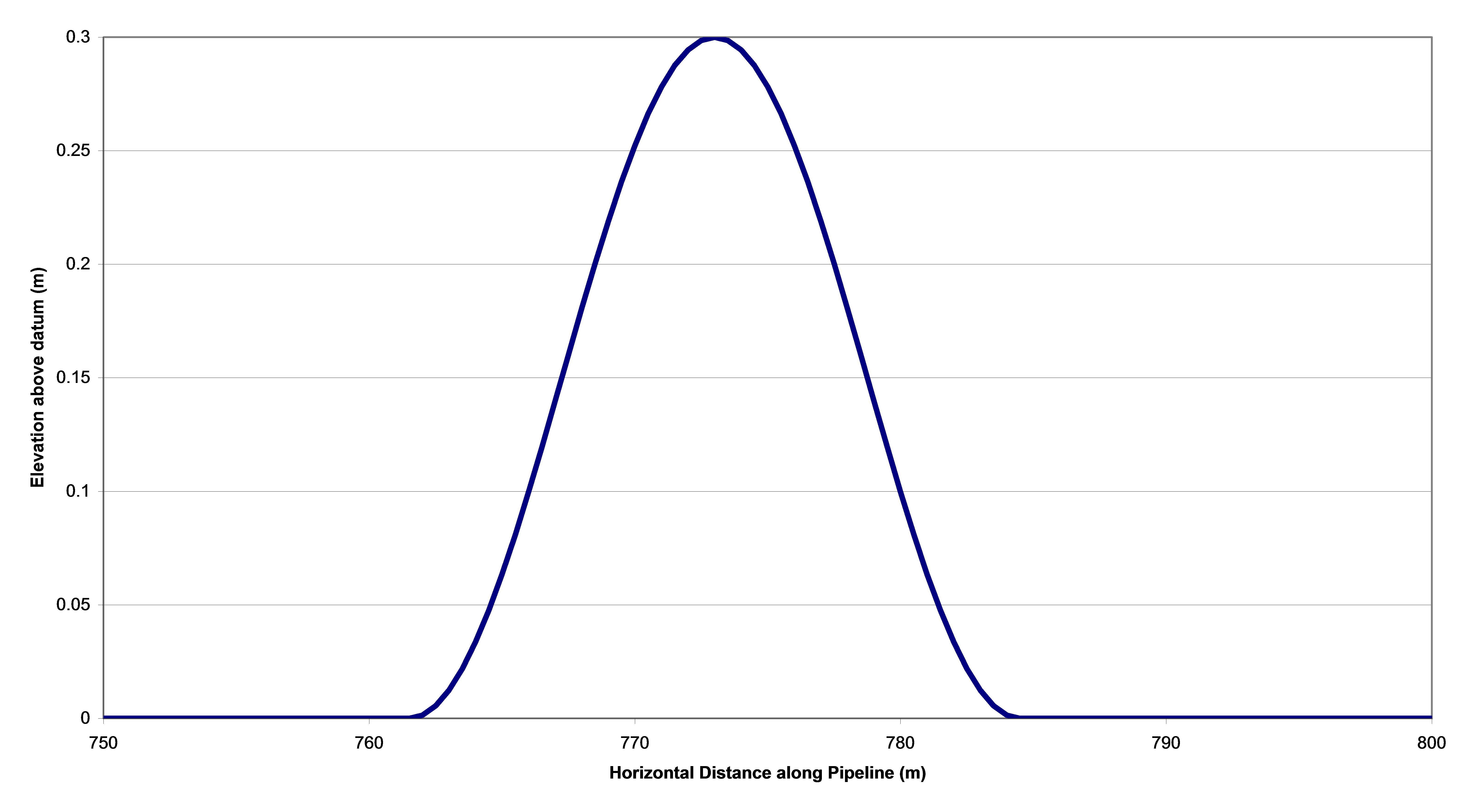
Seabed Imperfection Profile