Connected Mode, Normal Operating |
 
|
Connected Mode, Normal Operating |
|
Results from the connected mode analysis are presented in the following figures. The Static Effective Tension and Static Von Mises Stress figures below are from the static restart with offset and current, and plot respectively the distributions of effective tension and von Mises stress in the riser. The effective tensions are everywhere positive as required, and the stress values are acceptable. The discontinuity in the stress snapshot at approximately 4500 ft above the LFJ is due to the change in wall thickness here between joint Types #2 and #1 – the maximum von Mises stress clearly occurs at the inner circumference. Note that these figures, and indeed all snapshots and statistics plots presented hereafter, are for a user-defined set Riser which includes all riser joints between the lower flex joint and the telescopic joint, exclusive.
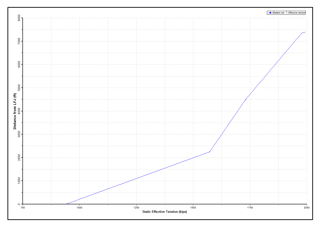
Static Effective Tension
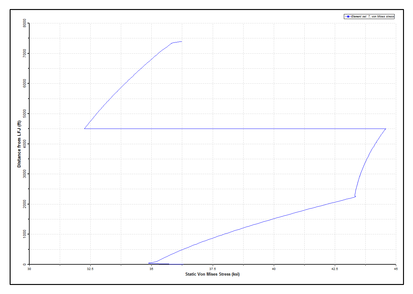
Static Von Mises Stress
The first figure below compares maxima and minima of riser rotation from the time and frequency domain solutions. The distributions show considerable agreement. The maximum predicted rotation at the LFJ is approximately 3.4 degrees for the time domain solution, and 3.3 degrees for the frequency domain solution. (In postprocessing the time domain results, statistics are generated over the last two wave periods). The second figure below compares the von Mises stress distribution along the riser from the time and frequency domain solutions. Again considerable agreement is observed. The time domain solution shows that the dynamic variation in stress is small, since the values are dominated by the axial stresses due to top tension. The actual stress values are within acceptable limits.
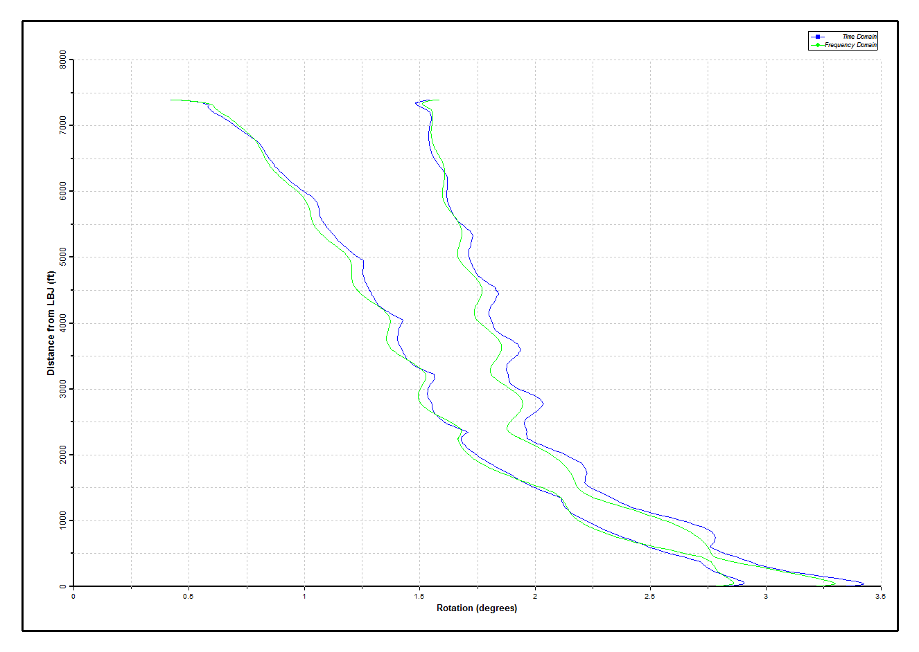
Comparing Rotations along Riser
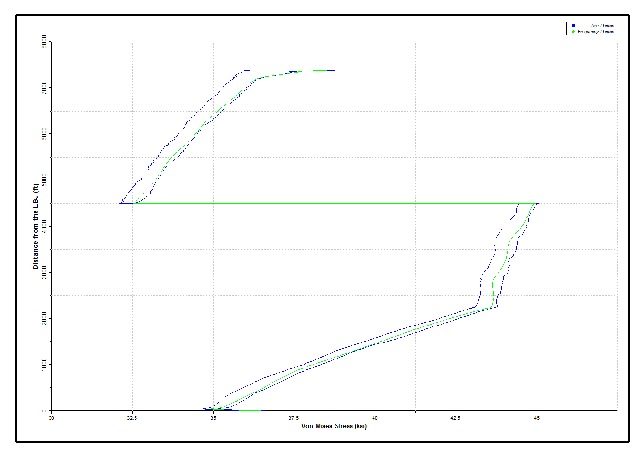
Comparing Von Mises Stresses along Riser
In figure 1-6, a maximum rotation at the LBJ of approximately 3.25 degrees is predicted by both time domain and frequency domain solutions. The distributions show considerable agreement. (In postprocessing the time domain results, statistics exclude the first 100 seconds of response, leaving a record of 2500 seconds for postprocessing). In the Comparing Von Mises Stresses along Riser figure below, the von Mises stress distribution is acceptable as before. Again there is excellent agreement between the distribution of von Mises stress predicted by the time domain and frequency domain approaches.
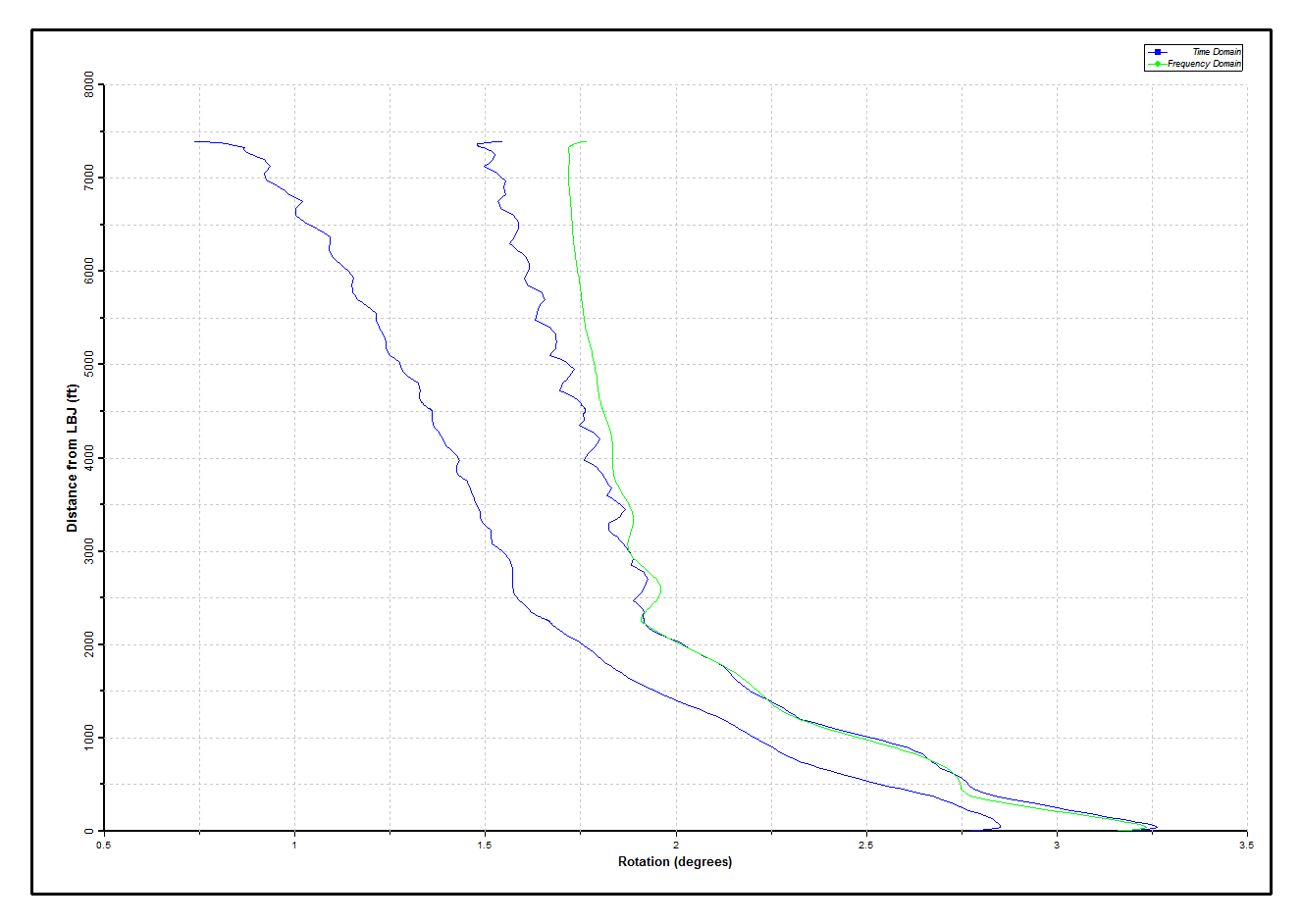
Comparing Rotations along Riser
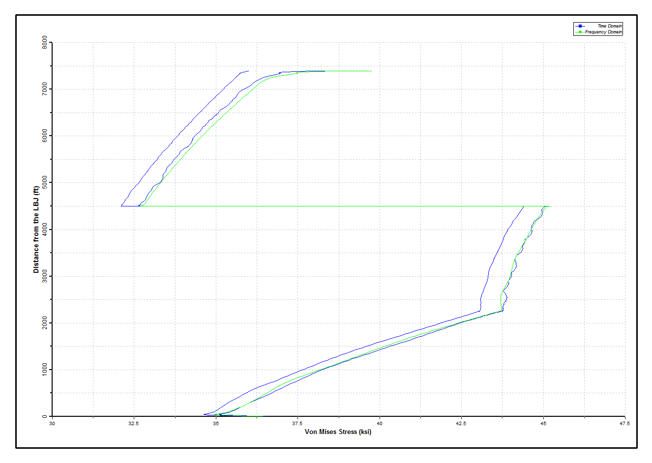
Comparing Von Mises Stresses along Riser
The table below presents the natural frequencies of the drilling riser in connected mode for the first 15 modes. For a TTR, pure bending modes are assumed to occur in identical or nearly identical pairs. So Modes searches for these pairs and categorises one of them as Bending and the other as Unknown.
The first figure below plots maximum curvature as a function of mode number (this plot is generated automatically by Modes). This type of plot is created to help in identifying so-called ‘mixed modes’ (refer to Modal Analysis for further information), where mixed modes tend to appear as local maxima or spikes. The maximum modal curvature should be monotonically increasing with mode number if pure bending modes only are considered.
Riser Natural Frequencies
Mode No. |
Period (s) |
1 |
78.03 |
2 |
36.59 |
3 |
24.09 |
4 |
18.44 |
5 |
14.73 |
6 |
12.12 |
7 |
10.42 |
8 |
9.19 |
9 |
8.12 |
10 |
7.26 |
11 |
6.64 |
12 |
6.09 |
13 |
5.59 |
14 |
5.19 |
15 |
4.86 |
One such spike is clearly identifiable in the first figure below, corresponding to Mode No. 21. This mode may be excluded from the Shear 7 output by invoking the TTR Modes – Exclude option, and the modal analysis may be performed again. As the objective this time is to recreate the Shear7 output only (a purely postprocessing option), the Repeat Run capability is utilised. This facility allows you to indicate that you do not want the program to redo the full eigensolution. Instead the program is to read the eigensolution details from an earlier run, but to recalculate the Shear7 data, in this case with certain modes excluded. The first figure below plots maximum curvature as a function of mode number, with the mixed mode excluded. The maximum curvature is now monotonically increasing with mode number, suggesting that only pure bending modes are now included in this output.
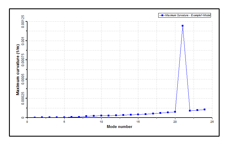
Maximum Curvatures
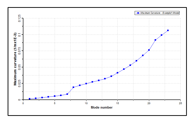
Maximum Curvatures, Excluding Mixed Modes
The figure below is a graph produced in Excel from tabular output presented in the output file. It plots the maximum curvature in each mode of the eigensolution, comparing the results at the element integration points, and the equal length segments used in the creation of Shear7 output. The intention here is to allow you to decide if you have specified enough segments to accurately capture the actual modal curvature distribution. In the present case the two sources agree reasonably well, so the specified number of segments appears reasonable.

Maximum Curvatures, Examining Segments
The below figure presents a summary of the fatigue analysis results.
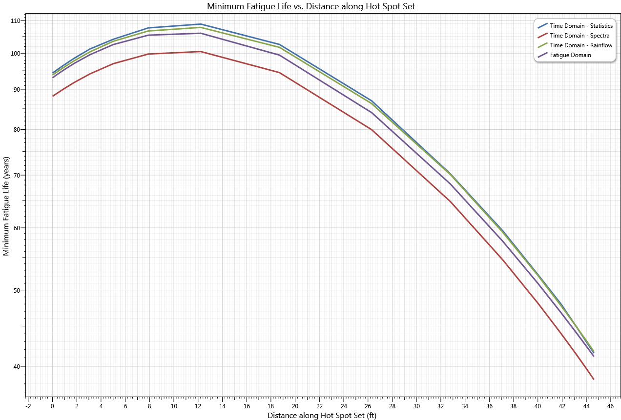
Fatigue Analysis Results
The lowest fatigue life occurs near the upper flex joint. The LifeFrequency and LifeTime results show very close agreement, particularly in view of the differences between the estimates produced by the different methods used within LifeTime itself. Note also that the computational effort required by the two fatigue analyses differ dramatically (i.e. only a few minutes for the frequency domain simulation as opposed to a few hours for the time domain analysis).